It is hard to keep a handwritten household account book. But I still want to keep track of my finances by hand.
Do you have such a problem?
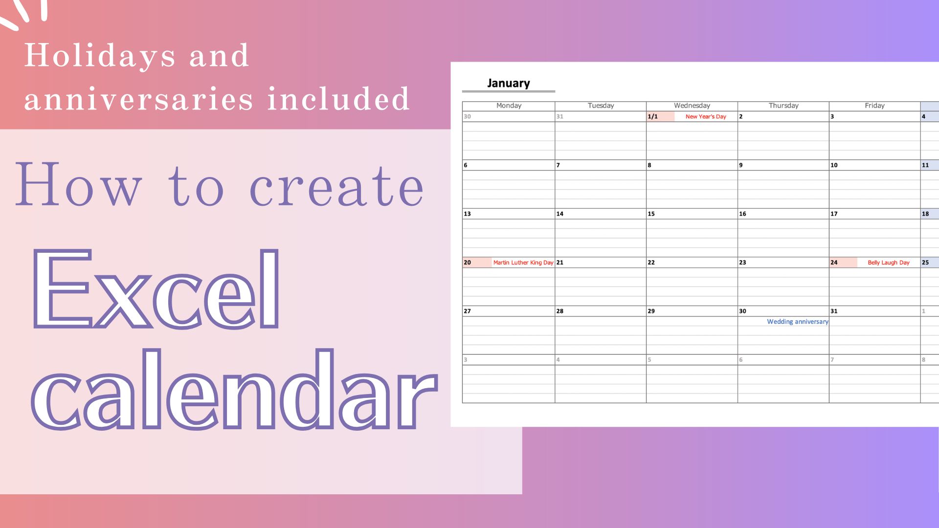
In this article, I will show you how to create a printable household budget calendar using Excel.
In any case, I will create a simple template that is easy to write and keep track of.
- Daily expense tracking
- Simple appointments and notes
- Monthly review
This calendar is designed to help you deal with your money while taking advantage of the benefits of handwriting.
This time, I will show you how to create a “variable expense calendar” only.
You can download a free template that allows you to manage items other than variable expenses here.
-
-
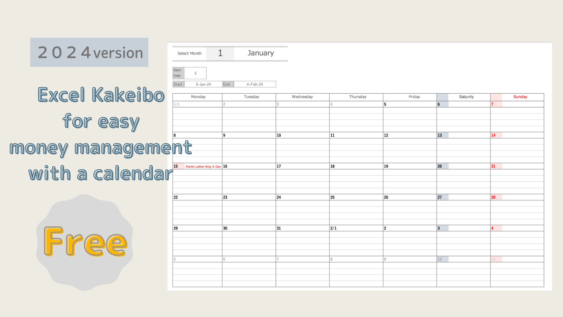
[2025 version] Excel Kakeibo for easy money management with a calendar "Free download"
It is hard to keep a handwritten kakeibo. But I still want to keep track of my finances by hand. Do you have such a ...
- Features of a Kakeibo Calendar
- How to Create a Kakeibo Calendar
- Create a new file
- Lists holidays and anniversaries
- Creating a Calendar
- Set Month
- Set Start Date
- Set calendar start and end dates
- Set calendar framework
- Set the date for Monday of the first week
- Setup for Sunday start
- Setting the date after Tuesday of the first week
- Holiday settings
- Set anniversary date
- Change background color for holidays
- Setting for dates when the date is 1
- Setting for weeks 2-6
- Set date before start date to gray
- Set date after end date to gray
- Hide start date, etc.
- Print settings
- Setting when the year changes
- Sample Templates
Features of a Kakeibo Calendar
- Can be created in Excel, printed out and used by hand.
You can manage your household budget as if you were writing on a piece of paper. - Holidays and anniversaries included
Holidays and anniversaries in your area are automatically displayed. Convenient for schedule management. - Start date can be freely set according to payday, etc.
You can adjust to your own life cycle instead of starting on the first day of each month. - Calendar format with one square per day
Designed for writing expense memos, appointments, and one-word diaries. - Simple and easy-to-read design
A clutter-free layout makes it easy to keep track. - One minute a day to record
Easy-to-use household account book that you can keep up with even if you are busy. - Manage your schedule, expenses, and notes on a single sheet
The calendar and the household account book are integrated. You can get a bird's eye view of the flow of your household finances.
How to Create a Kakeibo Calendar
Create a new file
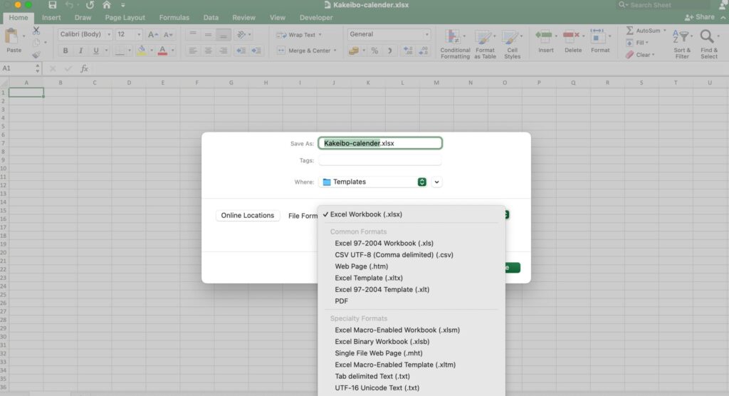
Open and name a new Excel file.
Click “Save As” on the file and create a “New Name”.
Select Excel Book (*xlsx) as the file type.
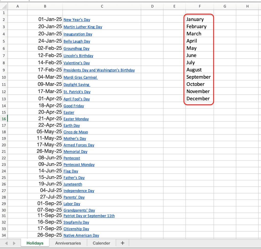
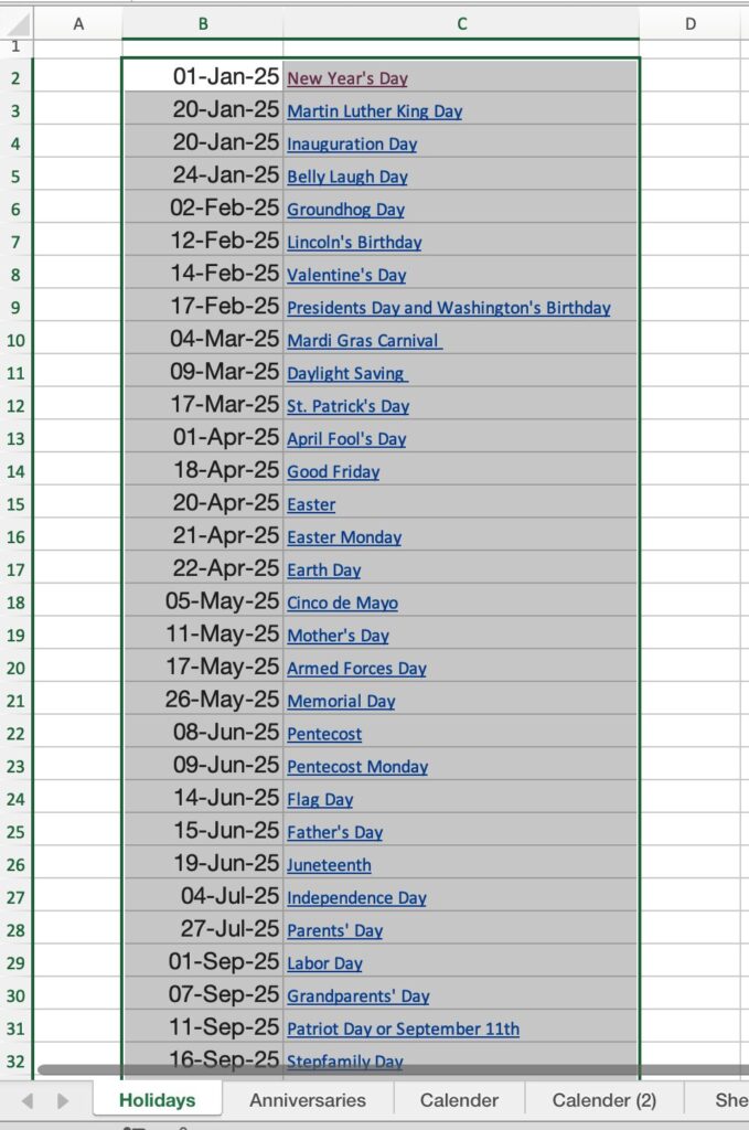
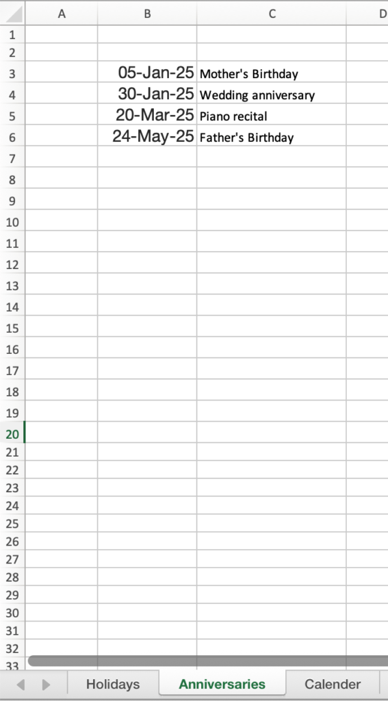
Lists holidays and anniversaries
Extracting Holidays
This setting is for displaying the names of holidays in the calendar.
Add a sheet and paste the list of holidays on a new sheet.
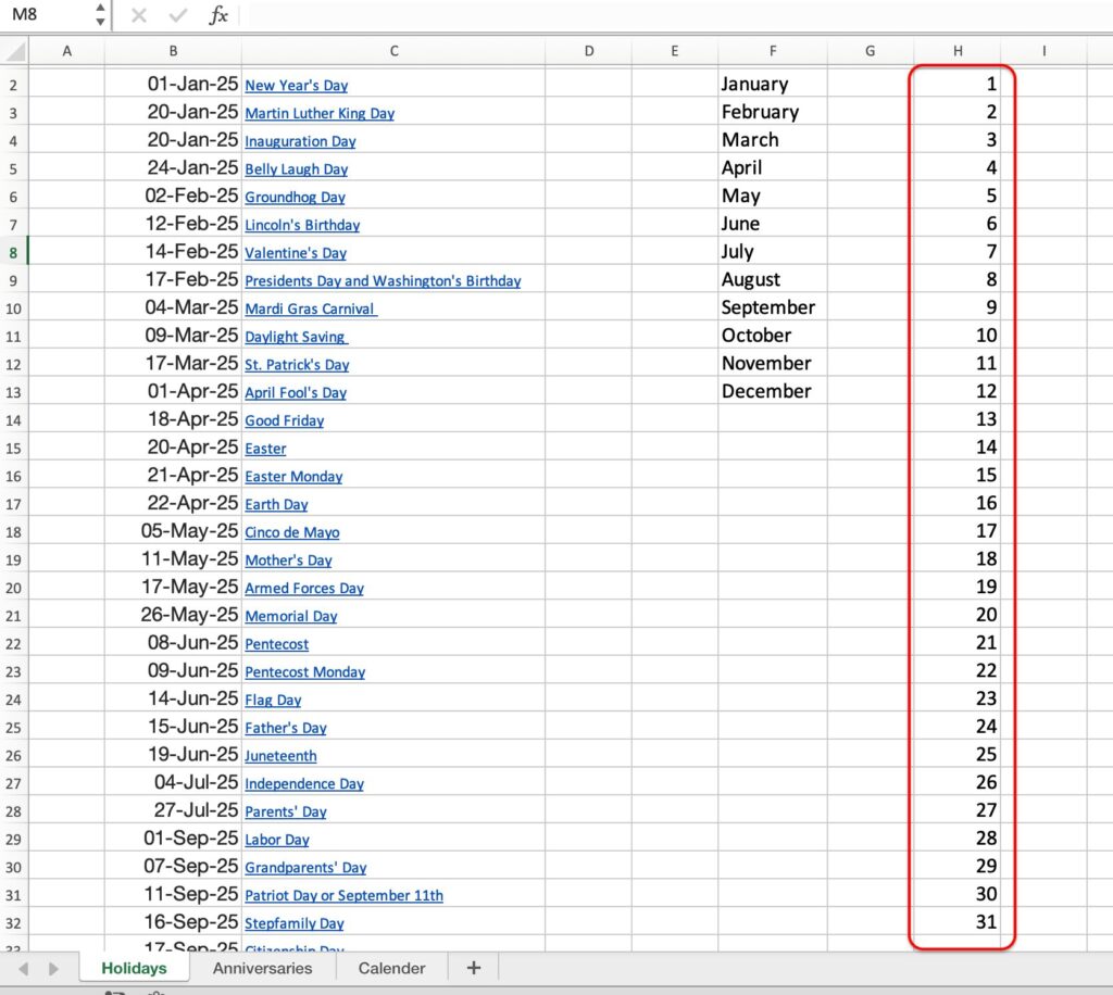
Using an internet search, search for “2025 Holiday List” and paste the date.
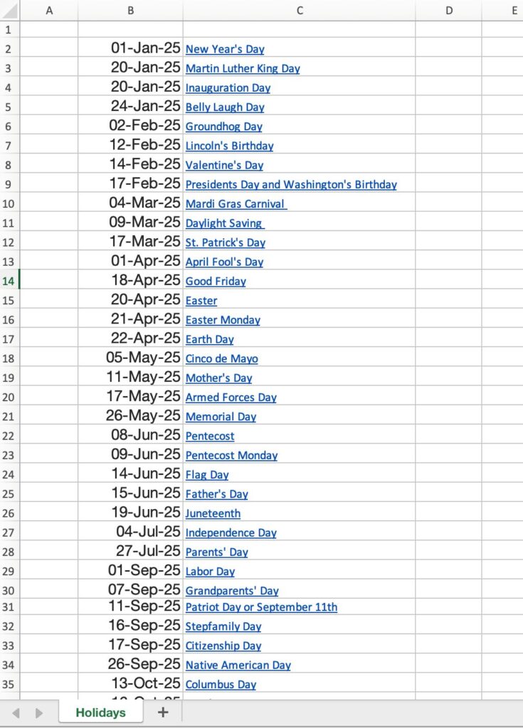
Please enter the year, month and day for the date.
Do not enter the day of the week.
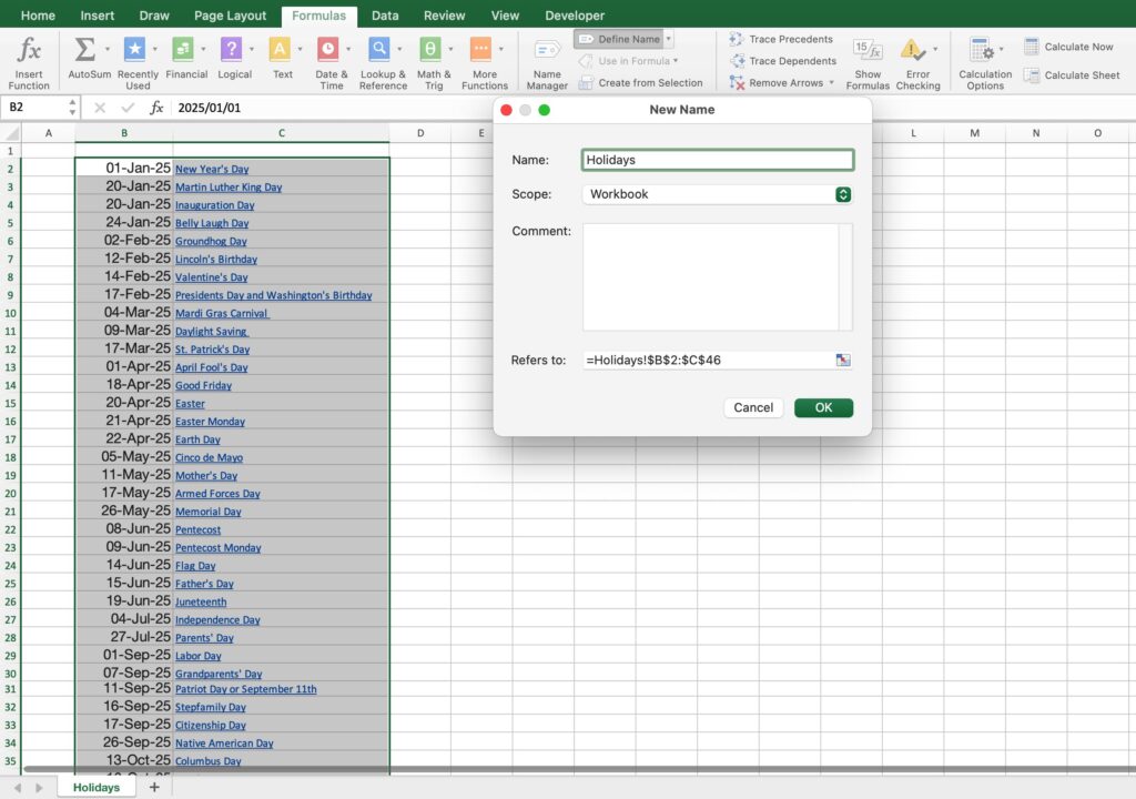
Name the list of holidays.
Names are required in calendar creation.
Select the Holidays list and choose Formula, Define Name.
Enter “Holidays” in the Name field.
List anniversaries
List anniversaries and appointments.
The anniversary date will appear in the calendar.
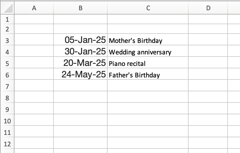
Please enter the year, month and day for the date.
Do not enter the day of the week.
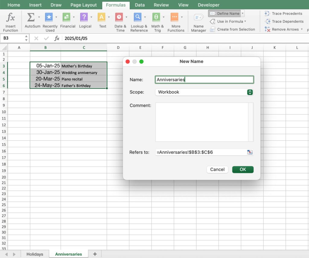
Name the list of Anniversaries.
Names are required in calendar creation.
Select the Anniversaries list and choose Formula, Define Name.
Enter “Anniversaries” in the Name field.
Creating a Calendar
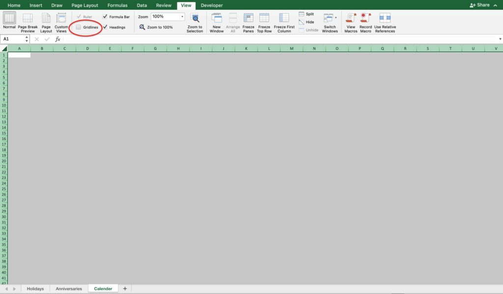
Add a sheet and name it “Calendar”.
Select the entire sheet (above the 1 in the upper left corner) and uncheck the Guidlines.
Set Month
There is one calendar sheet.
Select a month on the tab and set the calendar to display the calendar for the selected month.
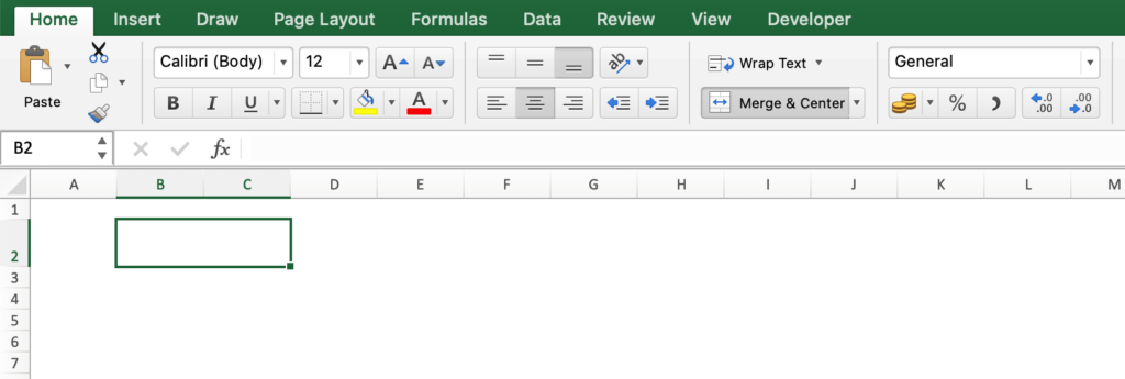
Select cell B2C2 and click on “Merge and Center Cells”.
Enter all months from January to December in the margins of the holiday list.
Select cell B2C2 and click on “Data Validation”.
Select “List” for Allow.
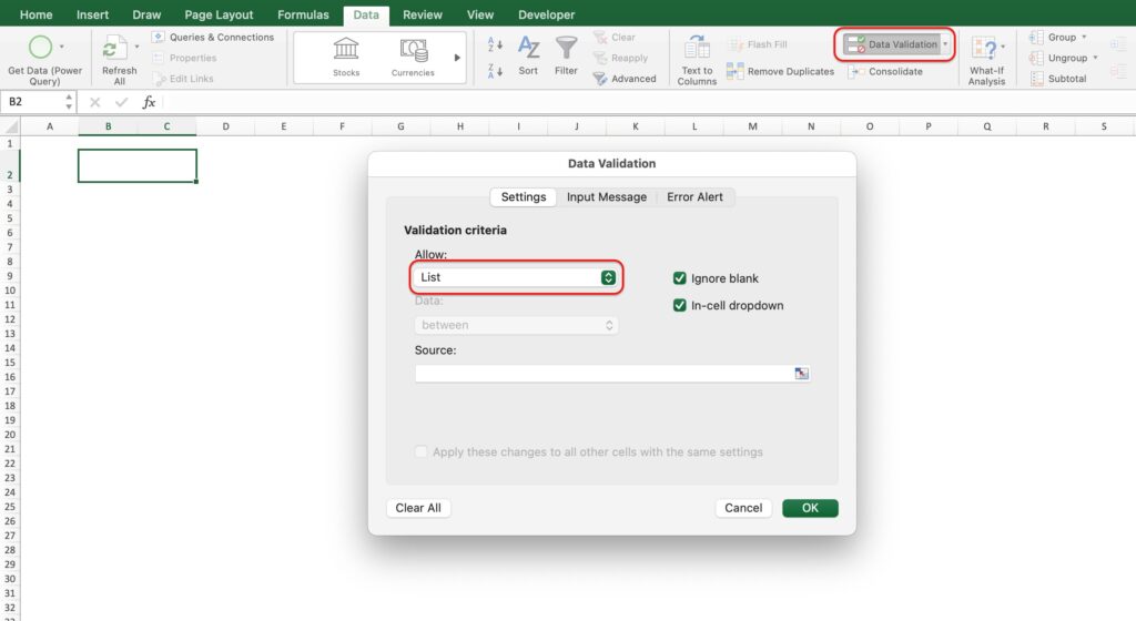
For the source, select the months January through December entered in the Holidays list.
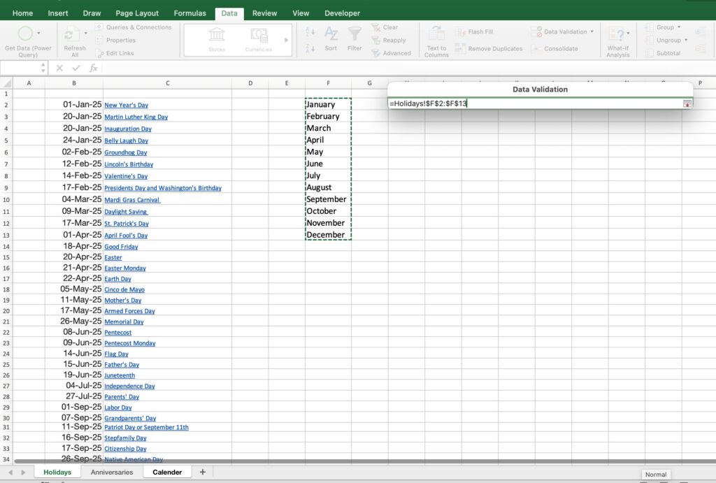
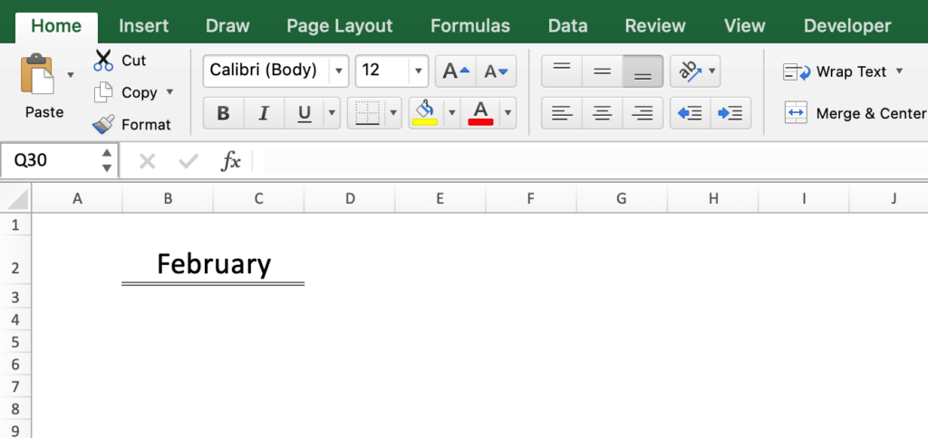
A tab has been added to allow selection from January through December.
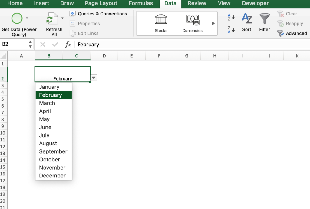
Change text color and text size if necessary.
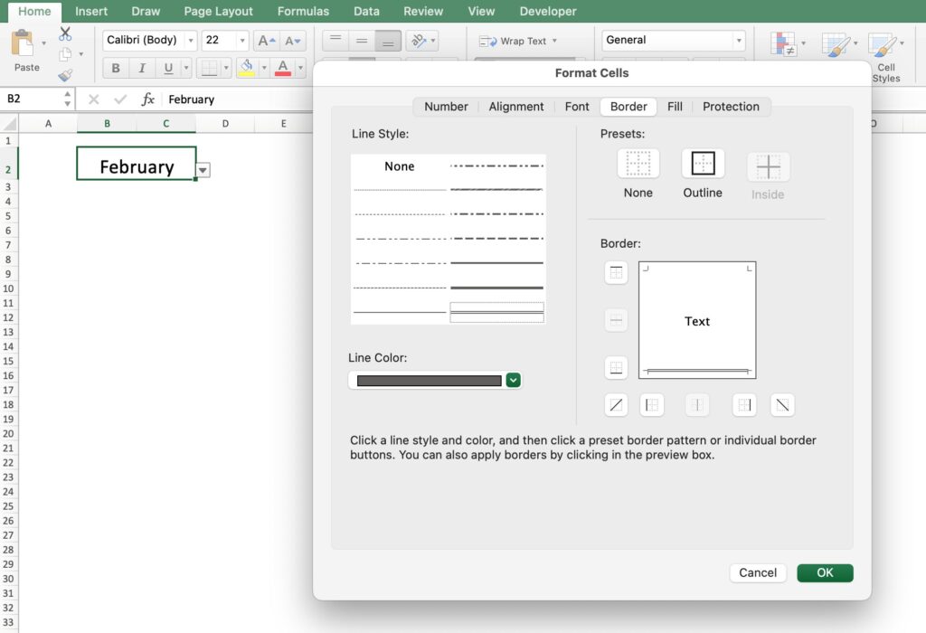
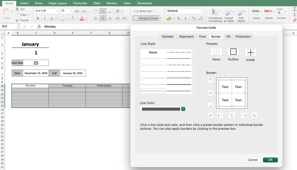
Add an underline from the cell formatting.
Select the Line style, Line color, and Border.
In the calendar start and end date settings, month names must be converted to numbers.
Since month names cannot be entered directly, months must be specified as numbers.
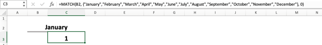
Use the Match function to convert month names to numbers.
=MATCH(B2, {"January","February","March","April","May","June","July","August","September","October","November","December"}, 0)
Set Start Date
Under Select Month, set the start date.
The start date allows you to set the start date of the month to coincide with your payday, etc.
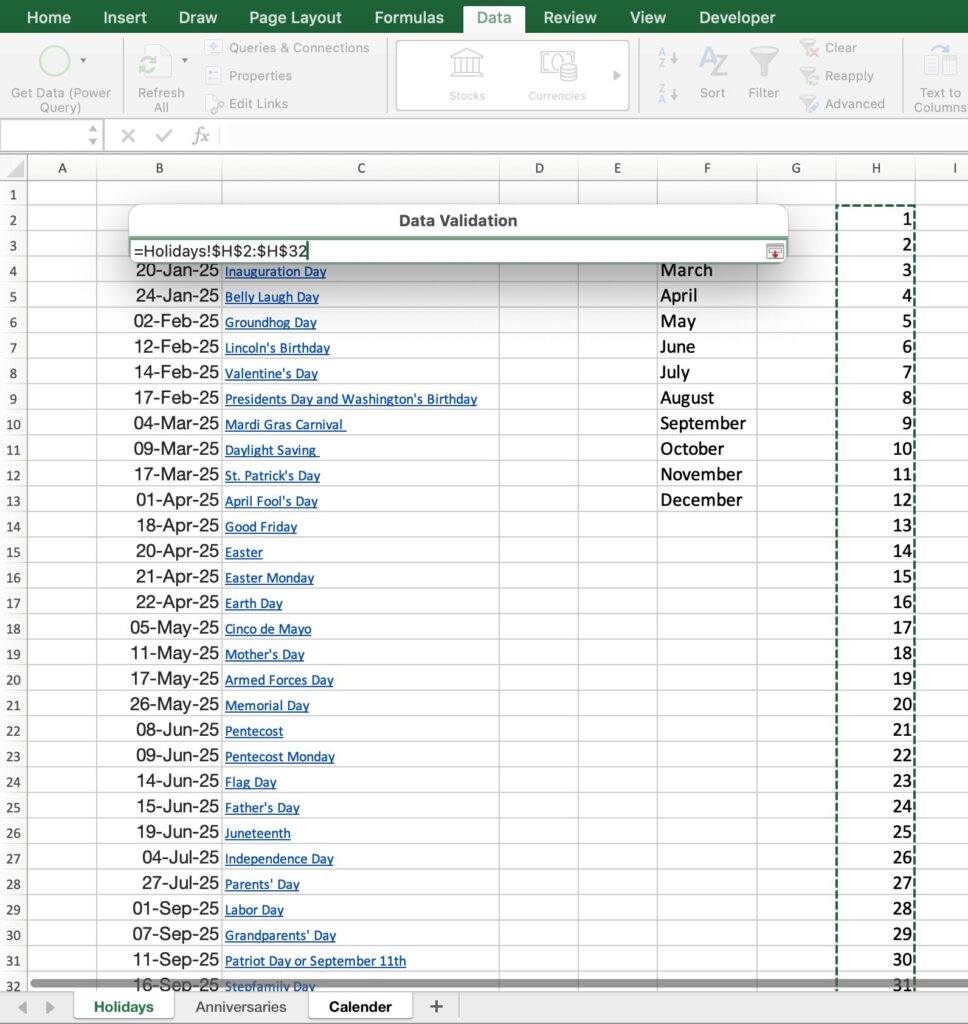
Enter a number from 1 to 31 in the margin of the holiday list.
Set the start date entry under the month.
Select the ”Data Validation” and select ”List” for Allow.
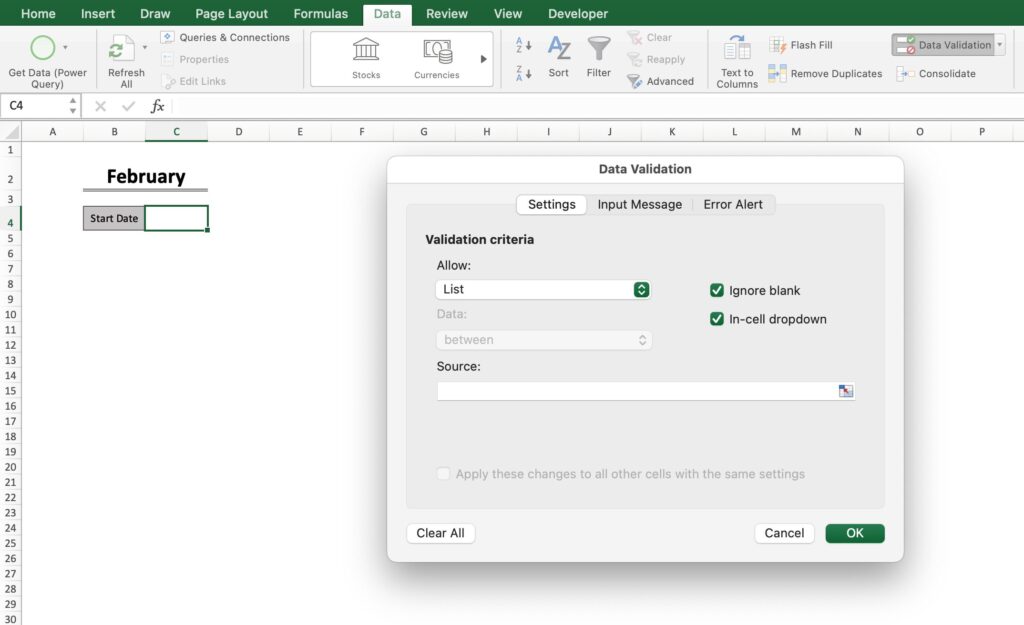
For the source, select a number from 1 to 31 in the list of holidays.
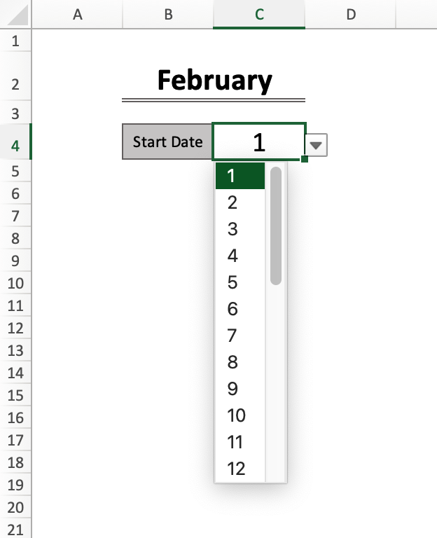
A tab will be set up for you to select a start date.
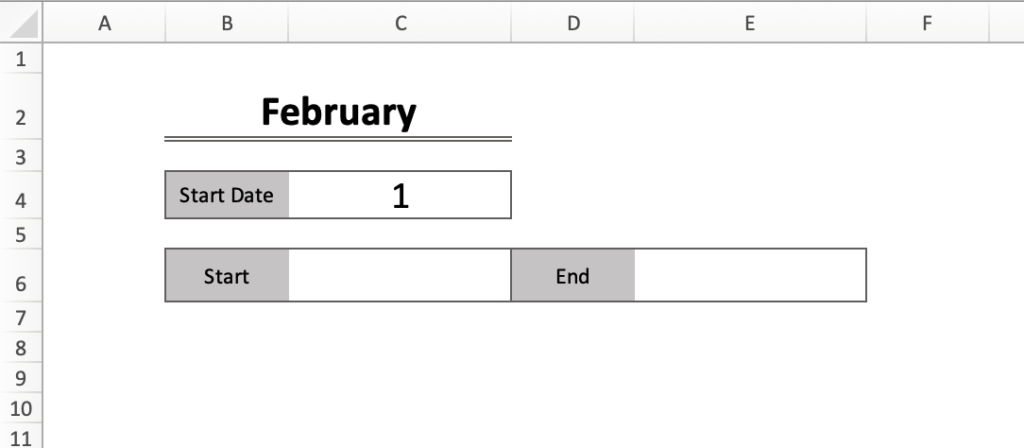
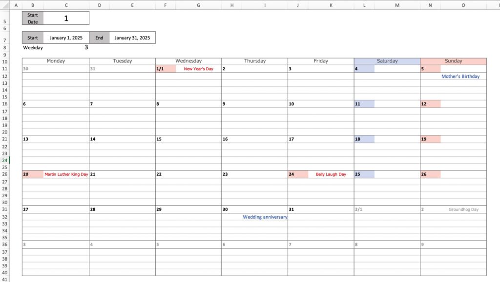
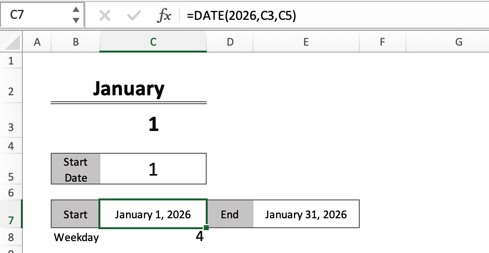
Set calendar start and end dates
Set the beginning and ending dates of the calendar.
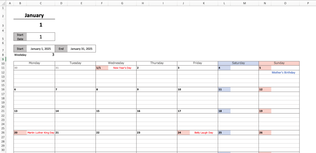
For example, if the month selection is “January” and the start date is “1,” the calendar will begin on January 1 and end on January 31.
After creating the framework, set the start and end dates.
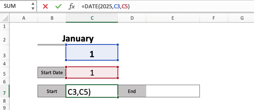
The DATE function is used to set the year, month, and date.
Set the year, month, and date using the rule “=DATE(Year,Month,Day)”.
The starting date is =DATE(2025,C3,C5).
Enter the current western calendar year for the year.
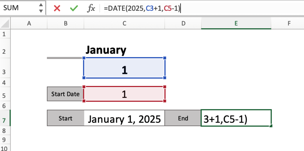
End date is =DATE(2025,C3+1,C5-1)
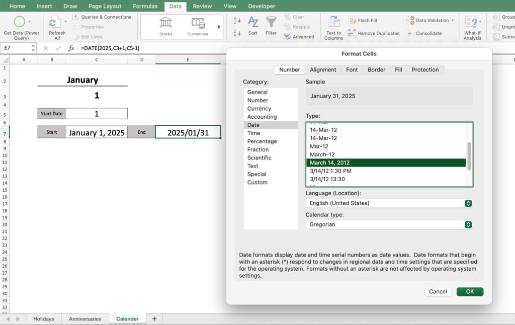
Right-click on the cell and select Formatcell; from Date, select the Type for the year, month, and day.
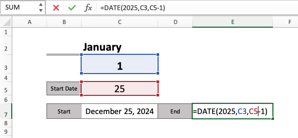
If the start date is later in the month and you want to start in the previous month,
- Start date: =DATE(2025,C3-1,C5)
- End date: =DATE(2025,C3,C5-1)
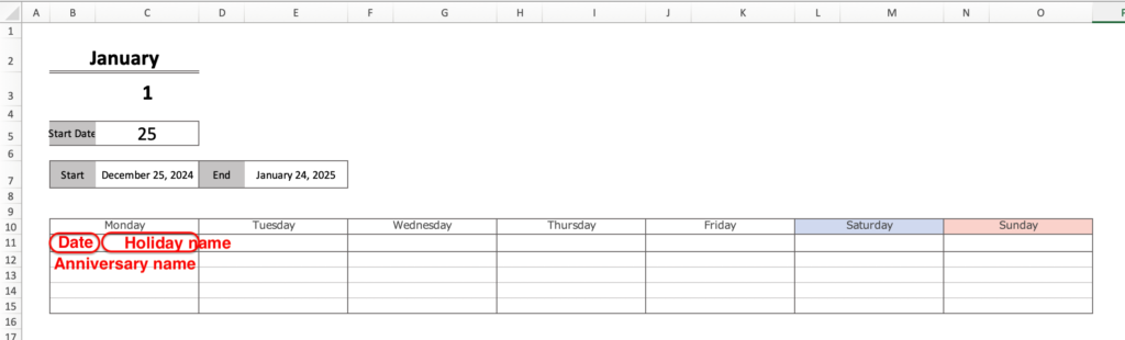
Set calendar framework
Create a calendar framework.
Copy and paste the first week's framework for the second and subsequent weeks.
Right-click on the range and select Format Cells.
Select the line style, line color, and border.
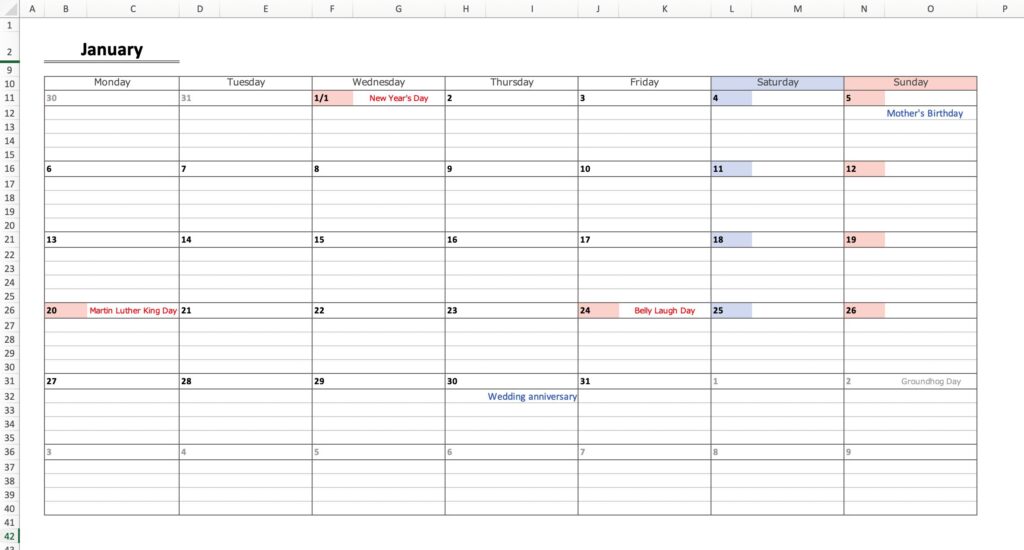
Line 11 displays the date and holiday name, and line 12 displays the anniversary name.
Set the date for Monday of the first week
First, we obtain the date of the first Monday of the first week.
To do this, we check what day of the week the start date is and find the date of the Monday of the same week.
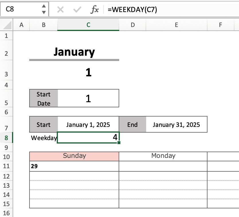
To check the day of the week, use the WEEKDAY function.
Insert one line under the start date and enter “=WEEKDAY(C7,2)”.
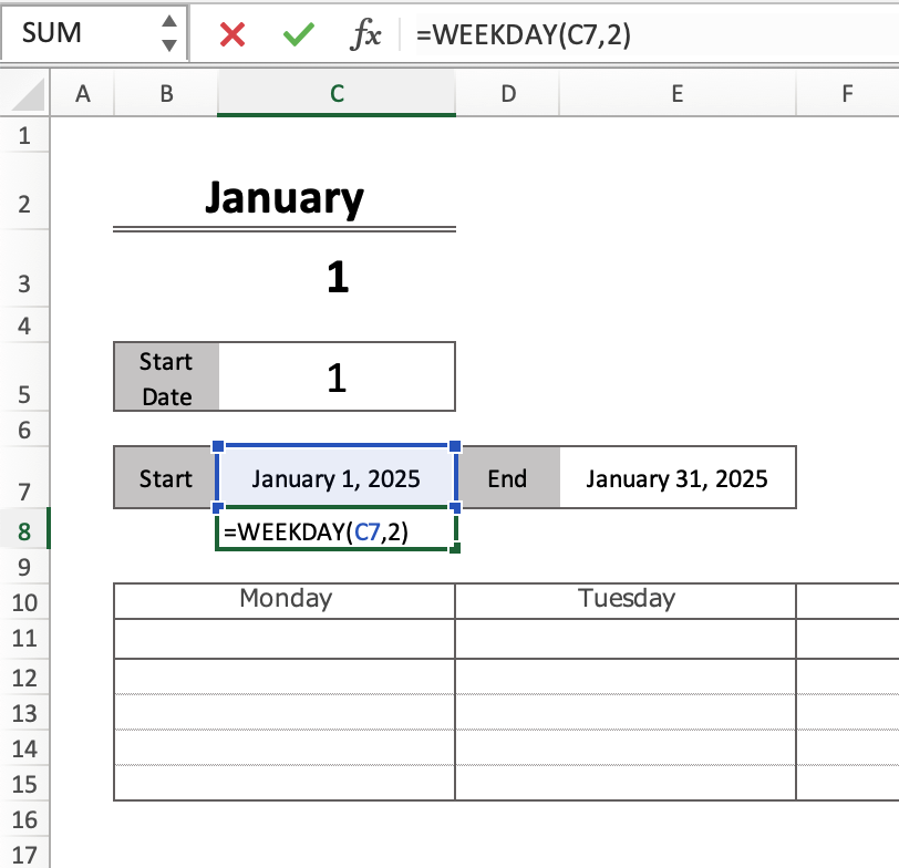
This calendar starts on Monday, so enter WEEKDAY( date ,2) so that Monday is 1.
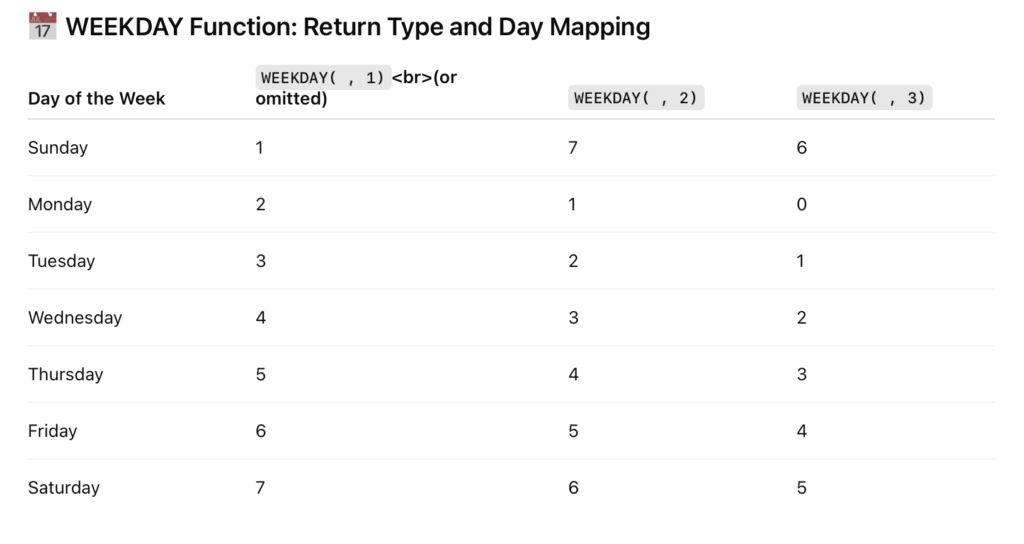
The day of the week on 1/1/2025 is indicated by a number.
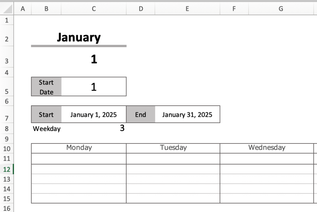
The date is displayed as 3, so it is Wednesday.
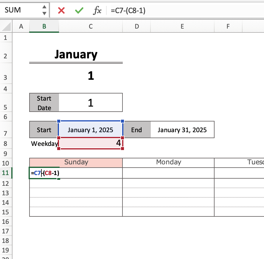
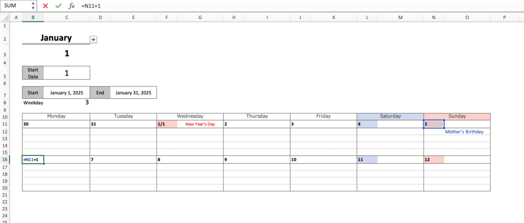
Monday's date is “Start Date - 2”.
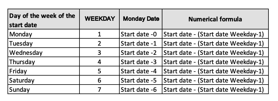
The formula is “=C7-(C8-1)”.
The start date is the start date with the year, month, and day.
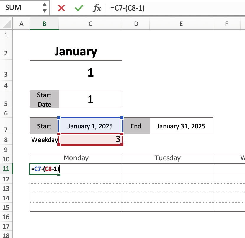
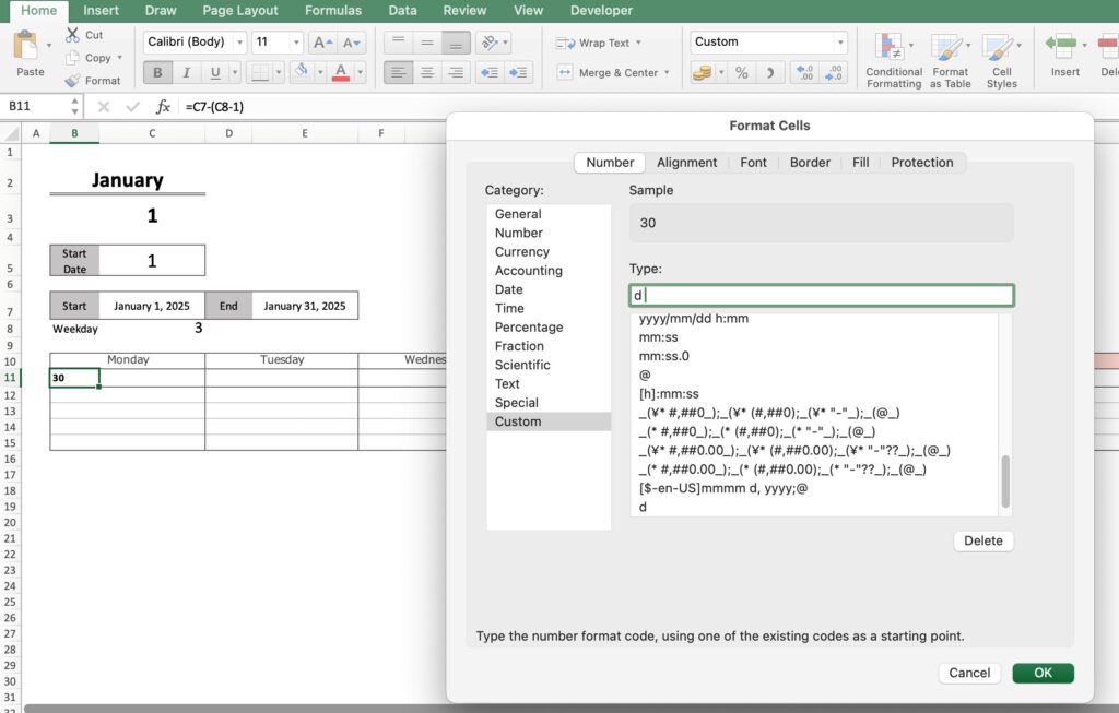
The date is displayed in the format of year, month, and day, so change it to show only the date.
Right-click on the cell and enter “Format Cells,” “Custom,” and “d” for the type.
Setup for Sunday start
Enter “=WEEKDAY(C7)” for the WEEKDAY formula for the start date.
The formula for Sunday dates is the same as for Monday beginnings.
=C7-(C8-1)
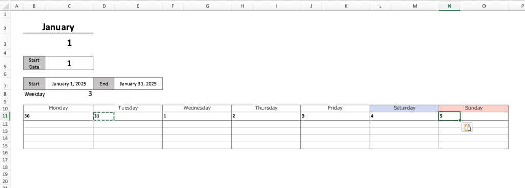
Setting the date after Tuesday of the first week
Tuesday's date will be “Monday's date + 1”.
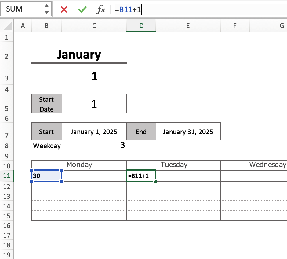
Copy and paste Tuesday's formula from Wednesday through Sunday.
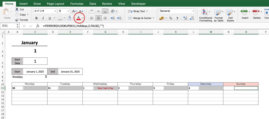
Holiday settings
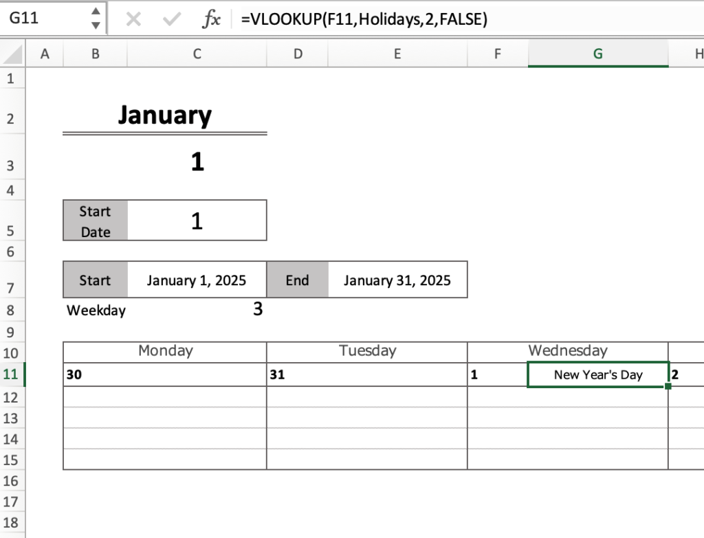
The name of the holiday is displayed next to the date using the VLOOKUP function.
The holiday names are taken from a “holiday list” created in advance.
The VLOOKUP function checks to see if there is a holiday in the holiday list that matches a date on the calendar, and displays the name of the holiday if there is one.
For example, if the date shown in “1” on the calendar is January 1, 2025, “New Year's Day” will be displayed next to it.
=VLOOKUP(value to look for, table range, column number, search method)
- Value to be searched: “1” of calendar (January 1, 2025)
- Range of table: B1:C32 of holiday list (*date and holiday name in holiday list)
- Column number: 2 (column with holiday name)
- Search method: FALSE (exact match: only if the dates match exactly)
Enter the formula in the cell next to the date
=VLOOKUP(H10,Holidays,2,FALSE)
The Holidays list range is named “Holidays”.
Enter “Holidays” instead of the range.
Entering this formula for an item that is not a holiday will result in an error.
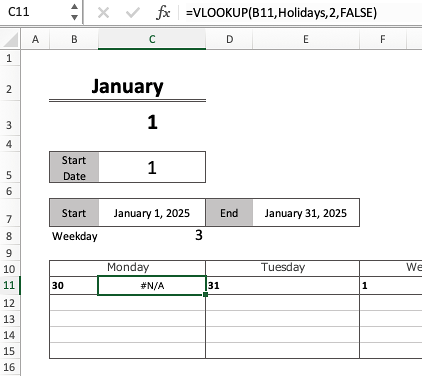
To avoid errors, add IFERROR before VLOOKUP.
The IFERROR function prints an alternative value when an error is displayed.
In this case, we want the error to be blank, so enter “=IFERROR(VLOOKUP・・・),"").
The “” is the symbol for blank.
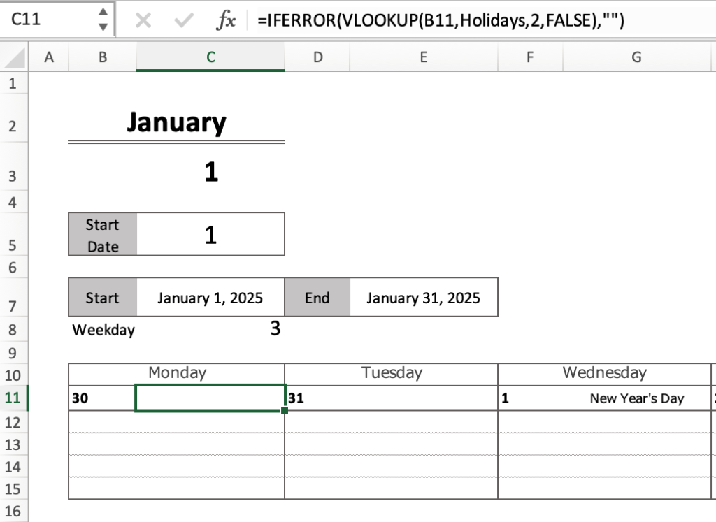
Paste this formula until Sunday.
After pasting, change the text color to red.
Set anniversary date
The VLOOKUP function is used to set anniversaries as well as holidays.
=VLOOKUP(value to look for, table range, column number, search method)
- Value to look for: “1” (January 1, 2025) in the calendar
- Range of table: B3:C6 of anniversary list (*Date and anniversary of anniversary list)
- Column number: 2 (column with anniversary date)
- Search method: FALSE (exact match: only if the dates match exactly)
Enter the formula in the cell in row 12.
=VLOOKUP(H10,anniversary,2,FALSE)
The anniversary list range is named “Anniversaries”.
Type “anniversaries” instead of the range.
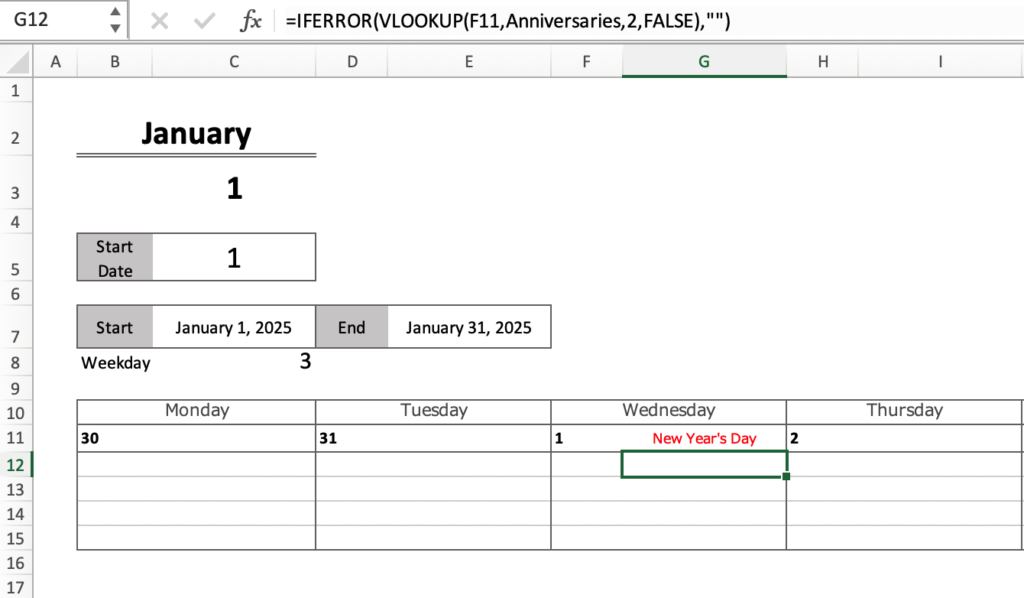
To avoid the error, add IFERROR before VLOOKUP.
The IFERROR function is a function that displays an alternative value when an error is displayed.
This time, we want the error to be blank, so we enter “=IFERROR(VLOOKUP・・・),””).
The “” is the symbol for blank.
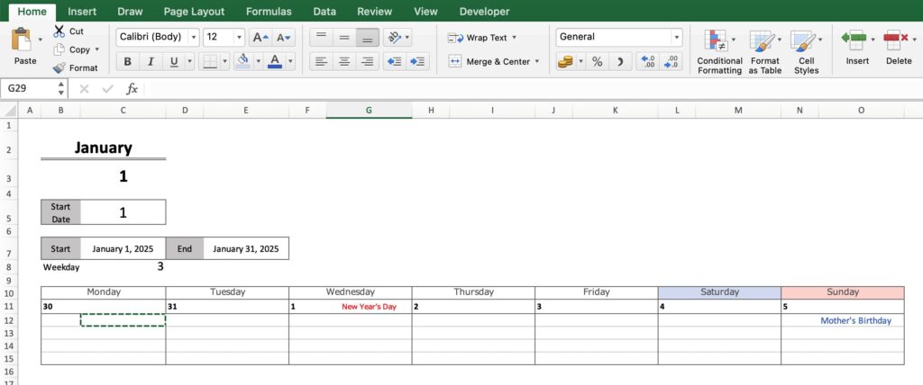
Paste the formula until Monday until Sunday.
Change the text color of the anniversary date if necessary.
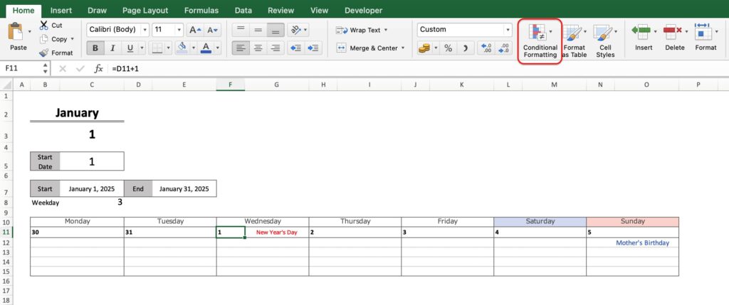
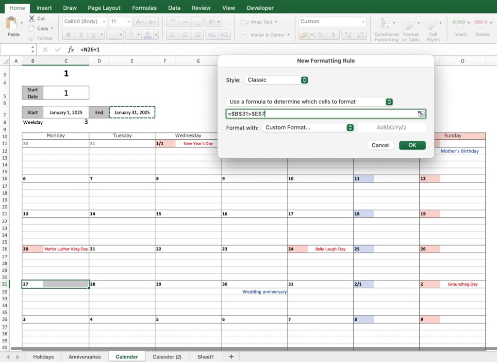
Change background color for holidays
Change the background color of the date to red to make it easier to recognize holidays.
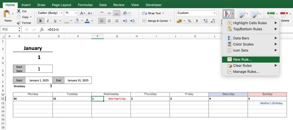
Click on a date cell and click on “Conditional Formatting”.
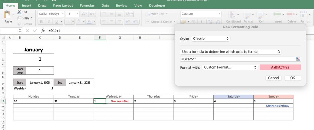
For Mac
- Style: Classic
- Use formulas to determine which cells to format
- Formula “=G11<>""
- Format: Custom Format
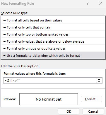
For Windows
- Use formulas to determine which cells to format
- Formula: =G11<>"”
- Select the Format and change the background color to red
Select red for the background color from Fill.
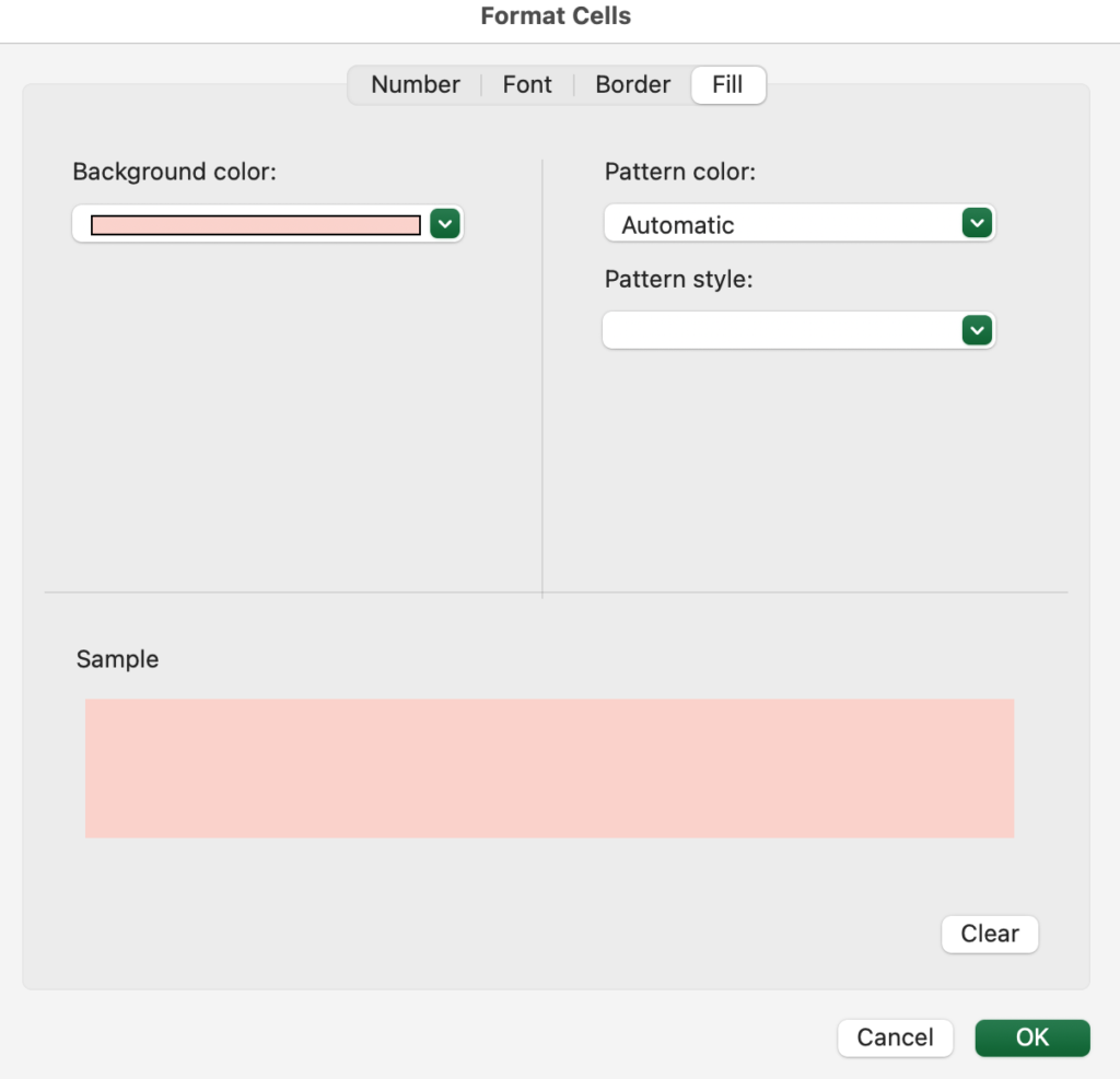
If you click on cell G11, you will see “$G$11”.
With the “$” attached like this, the cell reference is fixed when the cell is copied and pasted elsewhere.
If you want the reference cell to change according to where you copy it, remove the “$” and use “G11”.
When cell G11 is non-blank, set it to a bright red background color.
Symbol Description
<> other than
""Blank
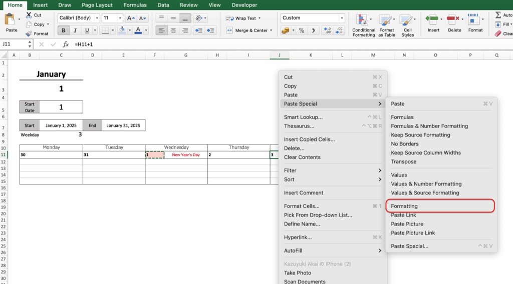
Copy cell G11 and select “Paste Format Only” for dates Monday through Sunday.
Paste all at once will change the range of conditional formatting.
Paste one by one.
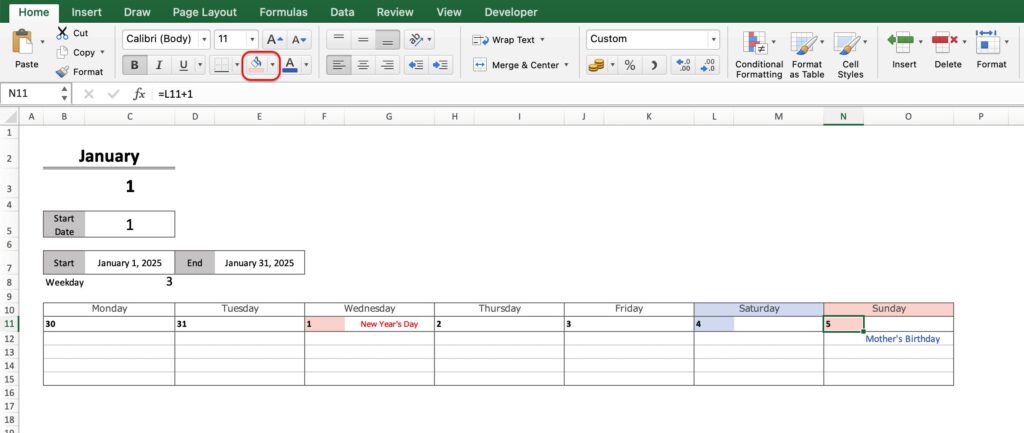
Please change the color to blue for Saturdays and red for Sundays from “Fill” on the home page.
If Saturday or Sunday falls on a national holiday, the color will automatically change to red.
Setting for dates when the date is 1
This calendar does not necessarily start with the date 1.
To give a visual indication when the month changes, only dates with a 1 will be displayed in a month/day format.
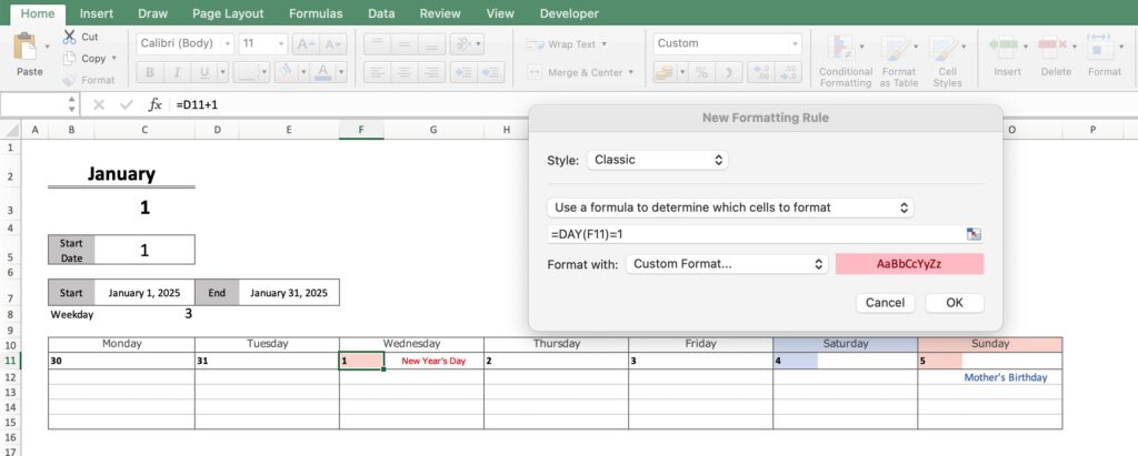
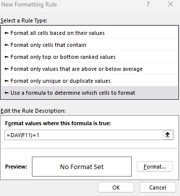
Select the date and click on “Conditional Format” and “New Rule”.
For Mac
- Style: Classic
- Use the formula to determine which cells to format
- Formula “=DAY(F11)=1
- Format:Custom Format
For Windows
- Use formulas to determine which cells to format
- “=DAY(F11)=1
If you click on cell F11, you will see “$F$11”.
With the “$” attached like this, the cell reference is fixed when the cell is copied and pasted elsewhere.
If you want the reference cell to change according to where you copy it, remove the “$” and use “F11”.
Cell F11 is 2025/1/1.
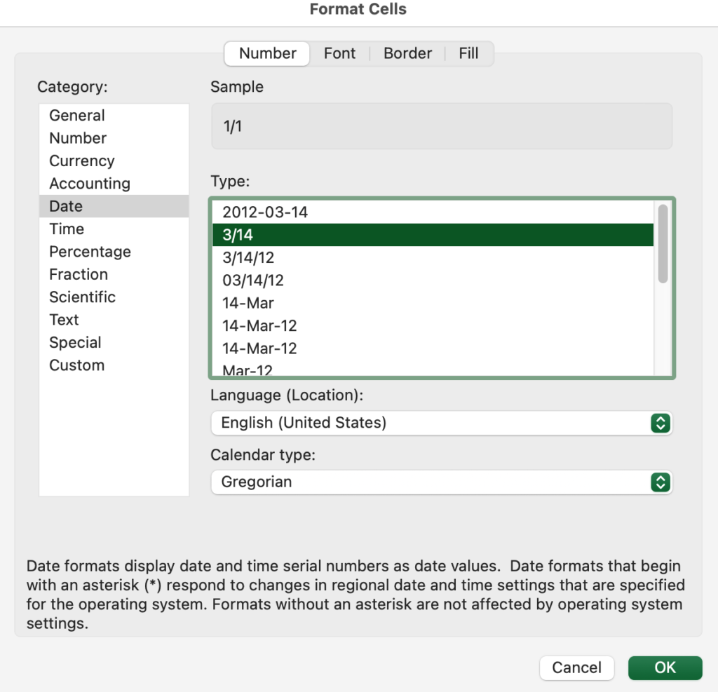
Use the DAY function to set conditional formatting when the date is 1.
Select “User-set formatting” to display the cell formatting.
Select “Month/Day” from Date in Display Format.
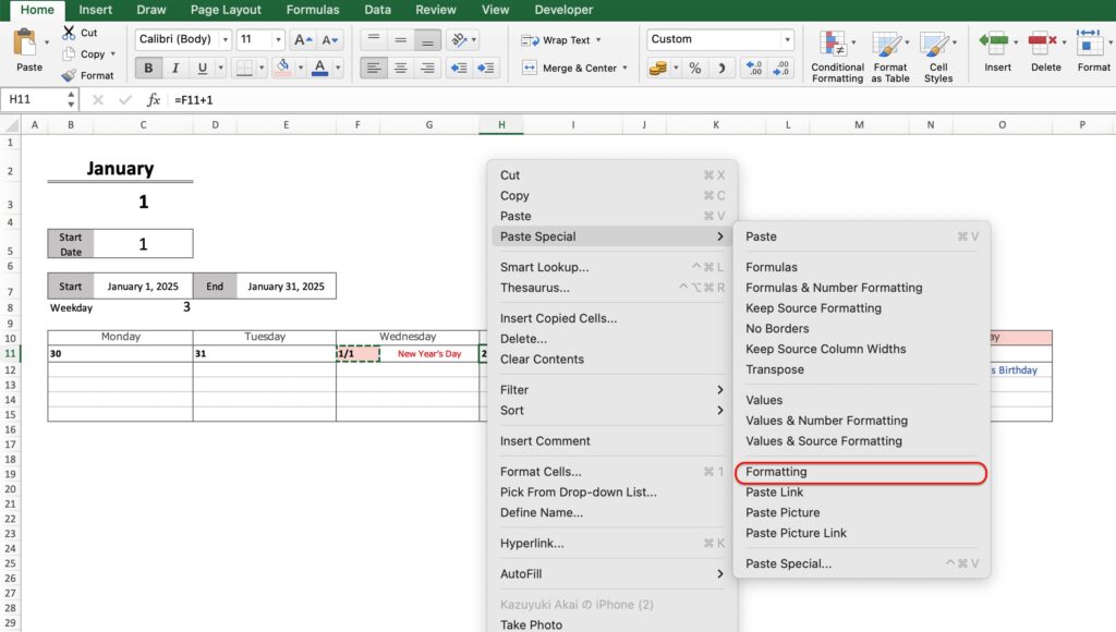
Copy cell F11 and select “Paste Format Only” for dates Monday through Sunday.
Pasting in bulk will change the range of conditional formatting.
Paste one by one.
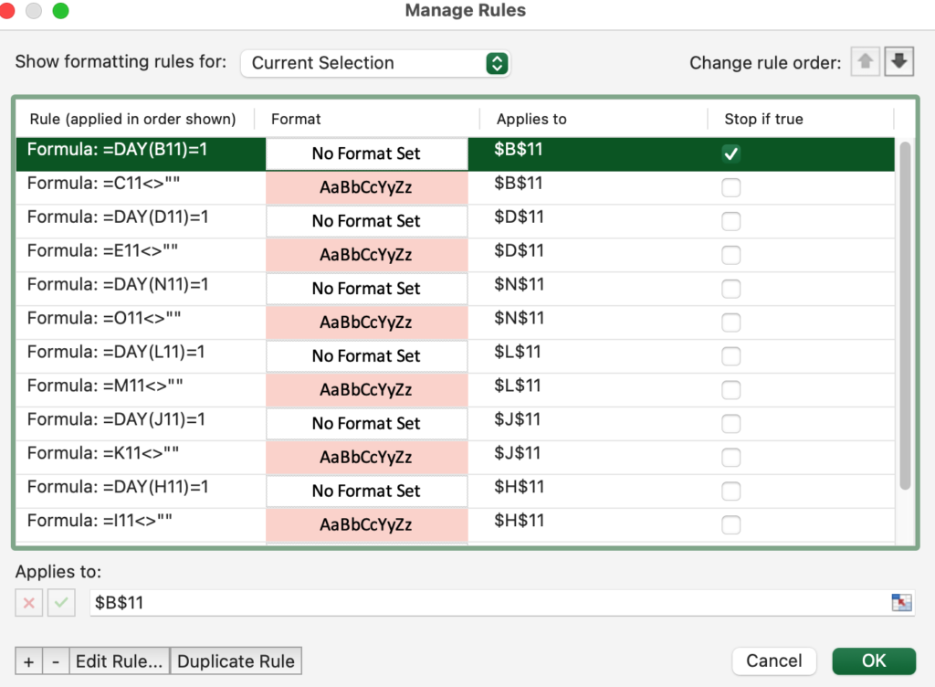
Conditional formatting can be modified from “Manage Rules” in “Manage Rules”.
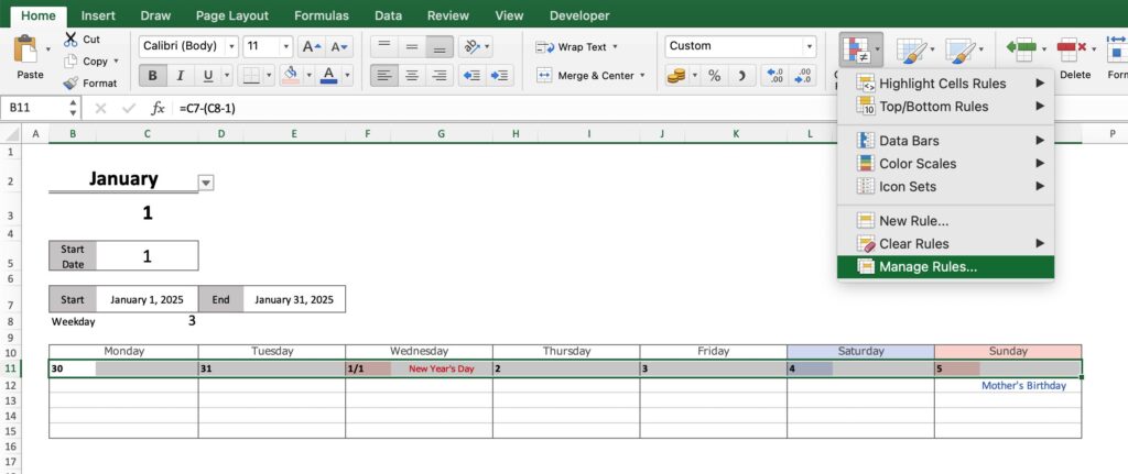
Double-click to see where to apply, formulas, and formatting.
Setting for weeks 2-6
Copy and paste the week 1 framework into week 2.
Correct the date of Monday of the second week to “the date of Sunday of the first week + 1”.
Copy and paste the framework from week 2 to weeks 3 through 6.
Set date before start date to gray
Gray the date before the start of the first week.
For example, if the 30th (2024/12/30) is before the start date (2025/1/1), the “Date, Holiday Name” will be grayed out.
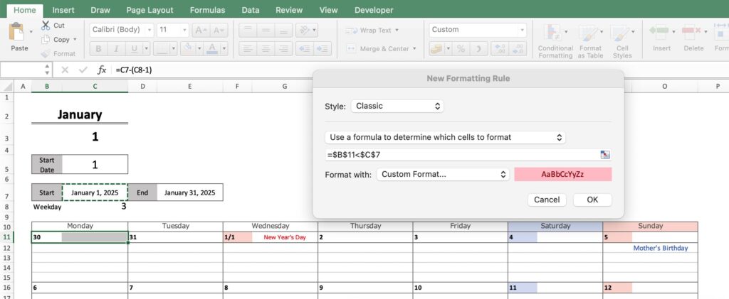
Select a range of dates and holiday names and click on “Conditional Formatting” and then “New Rule”.
For Mac
- Style: Classic
- Use formulas to determine which cells to format
- Formula “=$B$11<$C$7
- Format: Custom Format
For Windows
- Use formulas to determine which cells to format
- Formula “=$B$11<$C$7
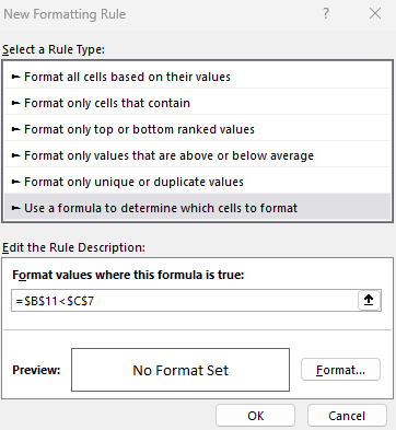
Cell B11 and cell C7 must be marked with a dollar sign.
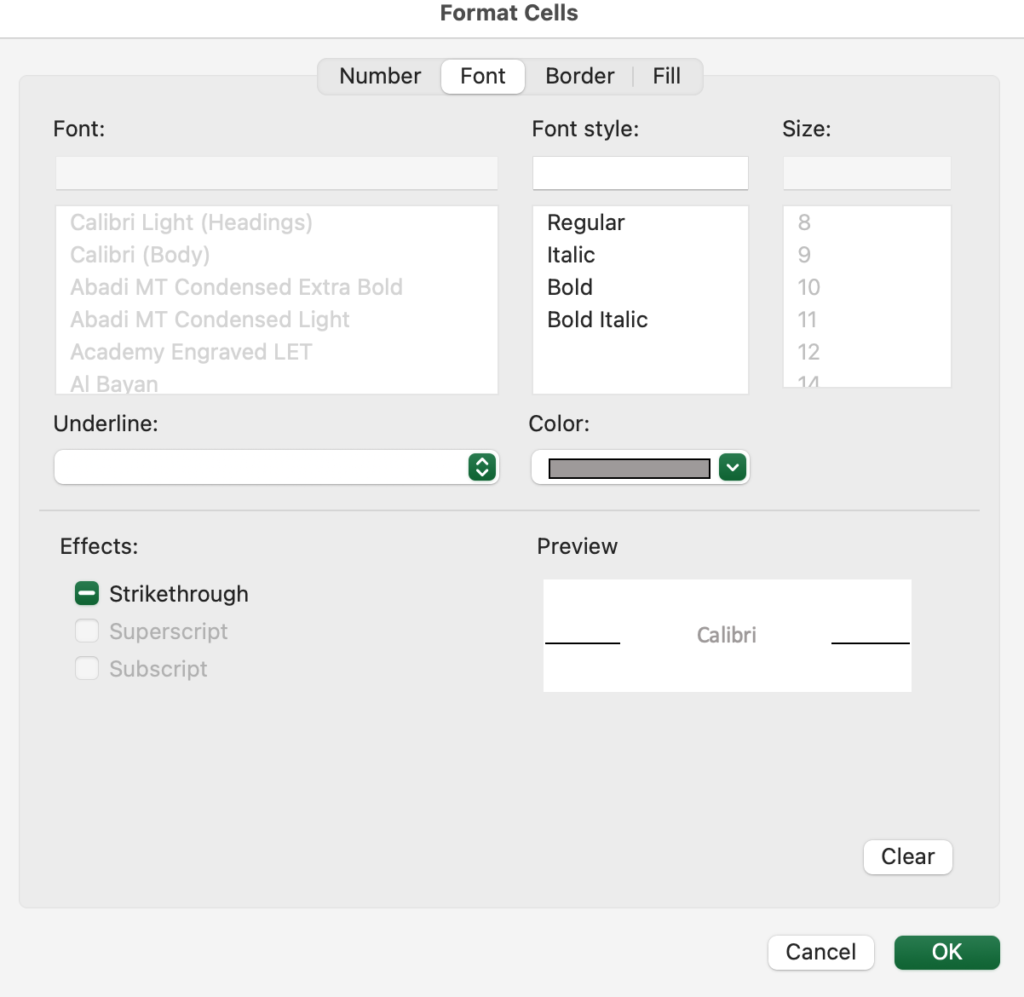
Set the “Font” color to “Gray” from the cell formatting.
Go to “Fill” and select “White” for the background color.
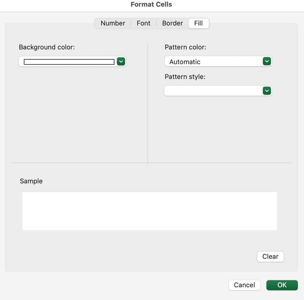
For dates before the start date, the text color changes to gray and the background color to white.
Since Sunday always contains a date after the start date, please use conditional formatting to set the range from Monday to Saturday of the first week.
Since the range is fixed with dollar signs in the conditional formatting, it cannot be copied and pasted.
Please set conditional formatting for each day.
Set date after end date to gray
The conditional format after the end date is set from Monday to Sunday of the 5th week 6th week.
(since February runs through the 28th).
Use the same method as for the gray setting before the start date.
The formula for conditional formatting is “=Date>End Date”.
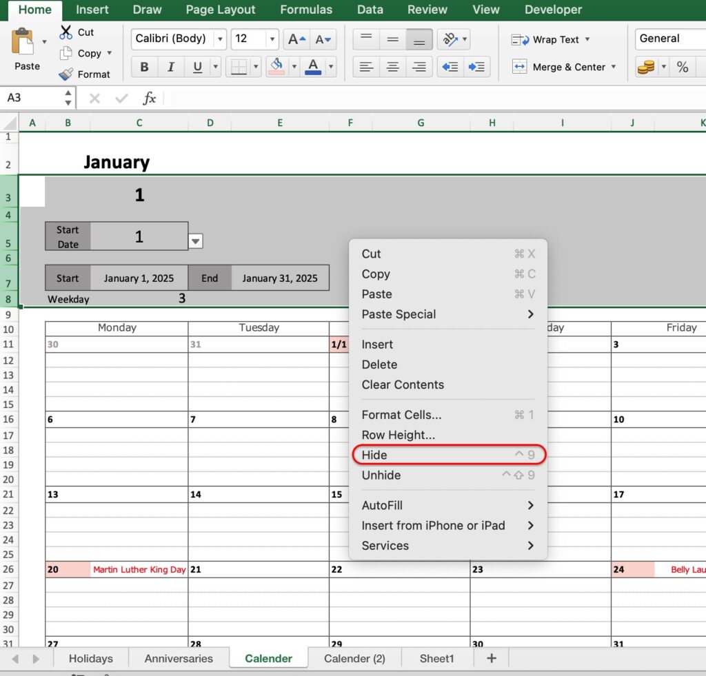
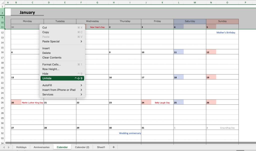
Hide start date, etc.
Right-click on the row you wish to hide and select “Do not show” or “Hide”.
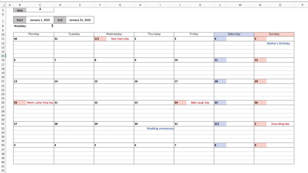
The calendar is complete.

Print settings
Select the area to be printed and click on “Set Print Range”.
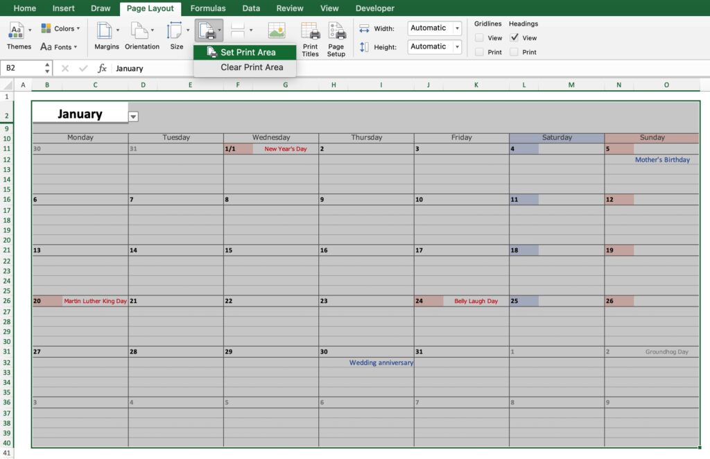
Select margins, print orientation, and size.
The print orientation should be landscape.
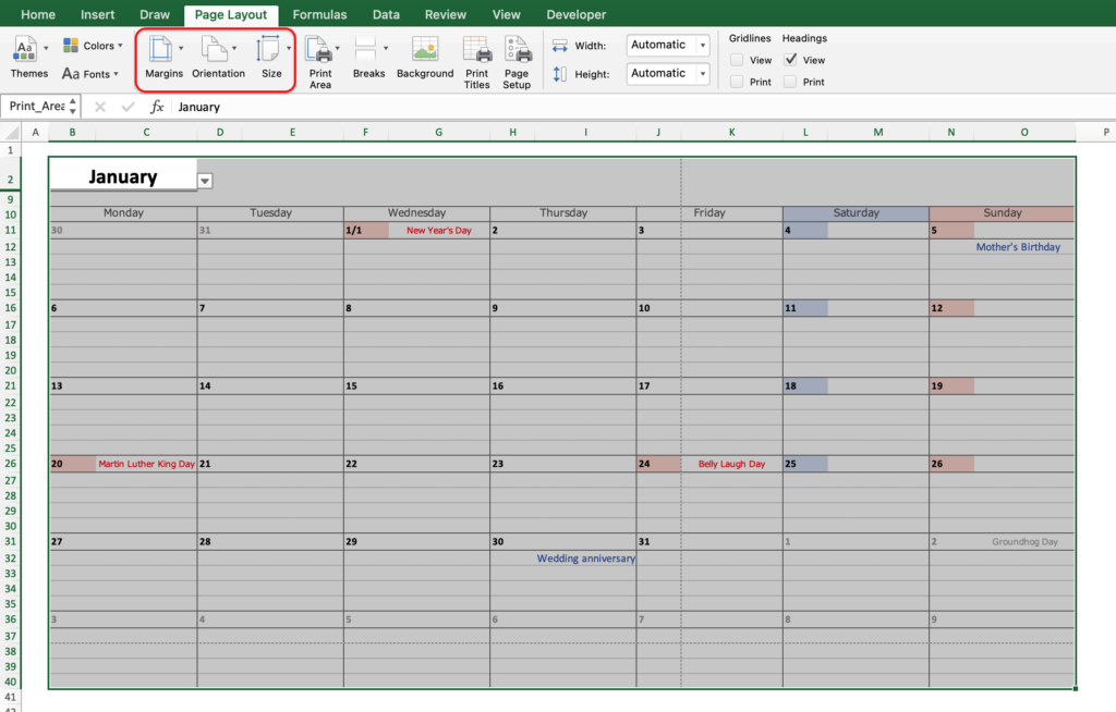
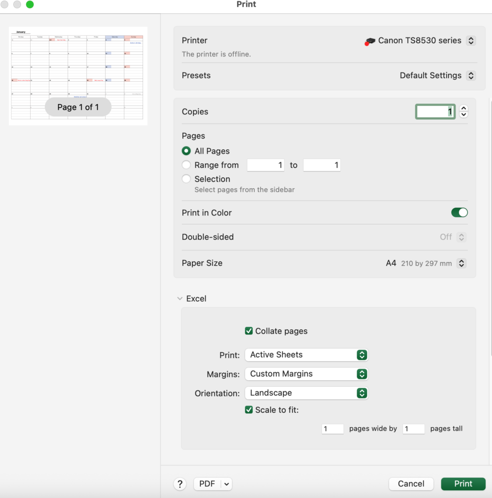
Please set the print area to fit on one sheet from the print settings.
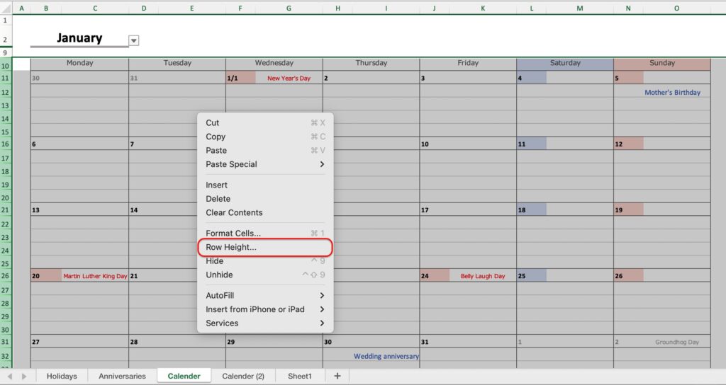
To change the column width, right-click on the target column and select “Column Width”.
Similarly, to change the height of a row, right-click on the target row and select “Row Height”.
Setting when the year changes
Paste the following year's holiday list to the previous year's continuation.
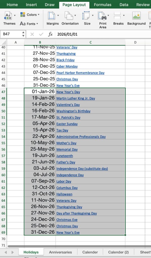
Select “Name Manager” under “Formulas.”
Add the following year's data to the reference range.
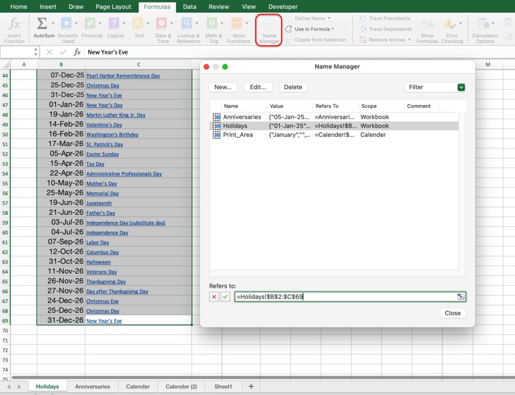
The anniversary date also changes the range in the same way.
Because the ranges are set up with names, the formulas for the anniversaries and holidays in the calendar do not need to be changed.
On the calendar sheet, change the start and end dates to the western calendar year.
To redisplay a hidden row, select the row, right-click, and choose ”Unhide.
Sample Templates
You can download a sample template from the button below.