I'd like to make my own, but I don't know how to do it...
On this blog, I'm currently distributing six different Excel household budgeting templates for free.(in Japanese)
In this article, I will explain the merits and demerits of Excel household account book, the points of making it, and how to make an Excel household account book, as revealed by creating various templates.
Advantages and Disadvantages of Excel Household Budgeting
Advantages
- Easy to tabulate.
- You can download templates almost for free.
- By creating your own, you can arrange it to suit your lifestyle.
- By creating graphs, you can easily compare and analyze the previous month's figures.
Disadvantages
- If you are not familiar with Excel, it is difficult to create your own.
- It takes time to start up the computer and open Excel.
- You downloaded a template, but it takes time to get used to the specifications.
- Can't find a household account template that fits my lifestyle.
Points to consider when making an Excel household account book
Clarify your purpose
The format you create will vary depending on whether you want to save money on food or keep track of your overall waste.
To save money on food
→Categorize the food expense items as staple food, side dishes, and favorite items.
To keep track of wasteful spending
→Color-code the items for wasteful spending to make it easier to see visually.If you want to understand your wasteful expenses, color-code the wasteful items to make them easier to see.
Consider for what purpose you want to create a household account.
Try to do as little as possible at a time
It is important to keep a household account.
It's hard to enter dates, expenses, contents, and amounts every time, isn't it?
Think about how you can make it easier by entering dates and expenses in advance.
Separate fixed costs from variable costs
Fixed expenses
expenses that must be incurred every month (housing, education, etc.)
Variable expenses
Expenses that occur every month, but the amount fluctuates.
By categorizing fixed expenses and variable expenses, you can find out whether your household budget is being squeezed by fixed expenses, variable expenses, or both.
Also, for variable expenses, setting a budget will make it easier to achieve your monthly goals.
Search for things you don't understand
You may have various questions such as how to use a function or how to add color.
In such a case, you can solve most of them by searching for "Excel, I want to add color".
I do a lot of searching...
Use graphs
One of the advantages of Excel is that you can use graphs as an analysis tool.
By using graphs, you can deepen your understanding.
Let's try to use graphs for month-to-month comparisons, expense ratios, etc.
Summary
- Clarify the purpose.
- Use only one operation at a time.
- Separate fixed costs from variable costs
- Search for things you don't understand.
- Use graphs
How to make an Excel household account book
Let's try to create a monthly sheet, an annual trend chart, and a graph by keeping the aforementioned points in mind.
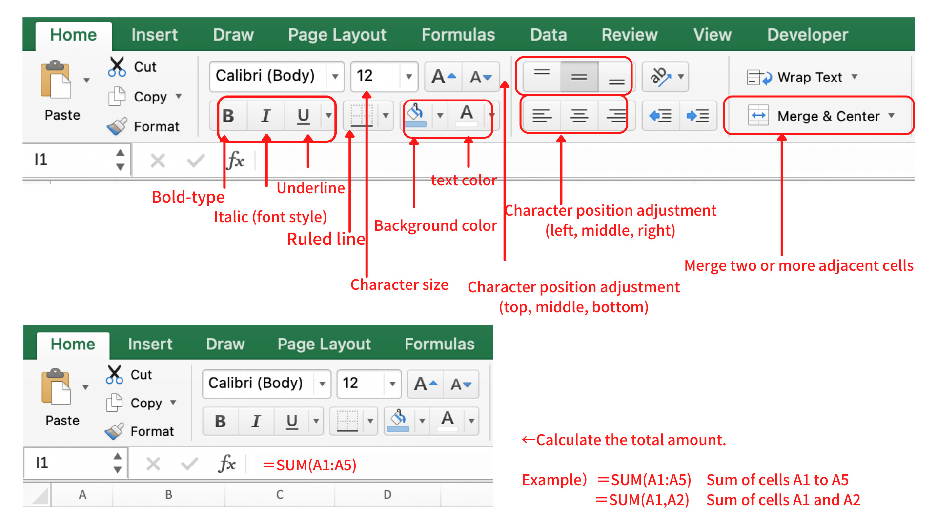
Basic Excel operations
Here is a summary of the basic operations used in creating an Excel household budget.
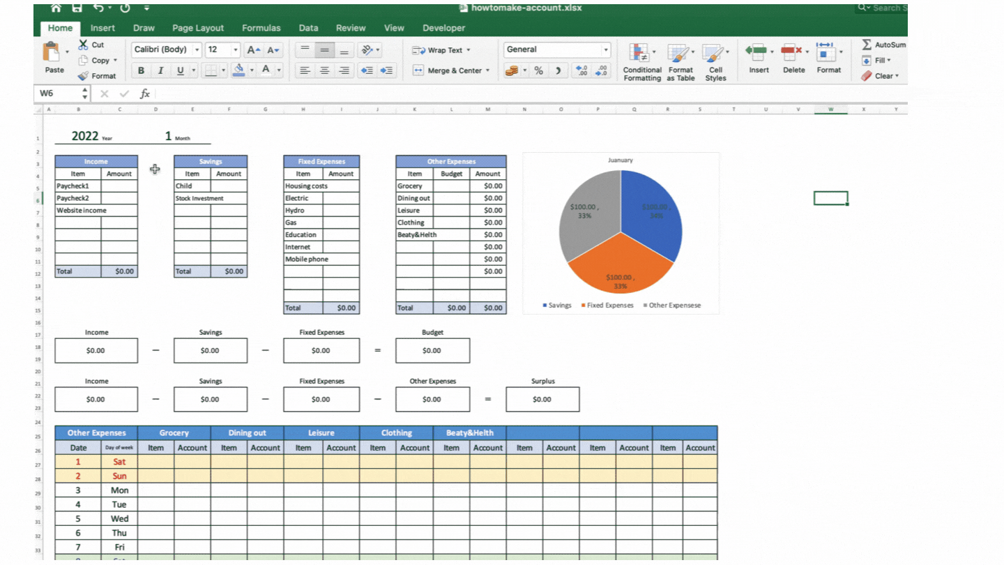
Monthly sheet
Completed image
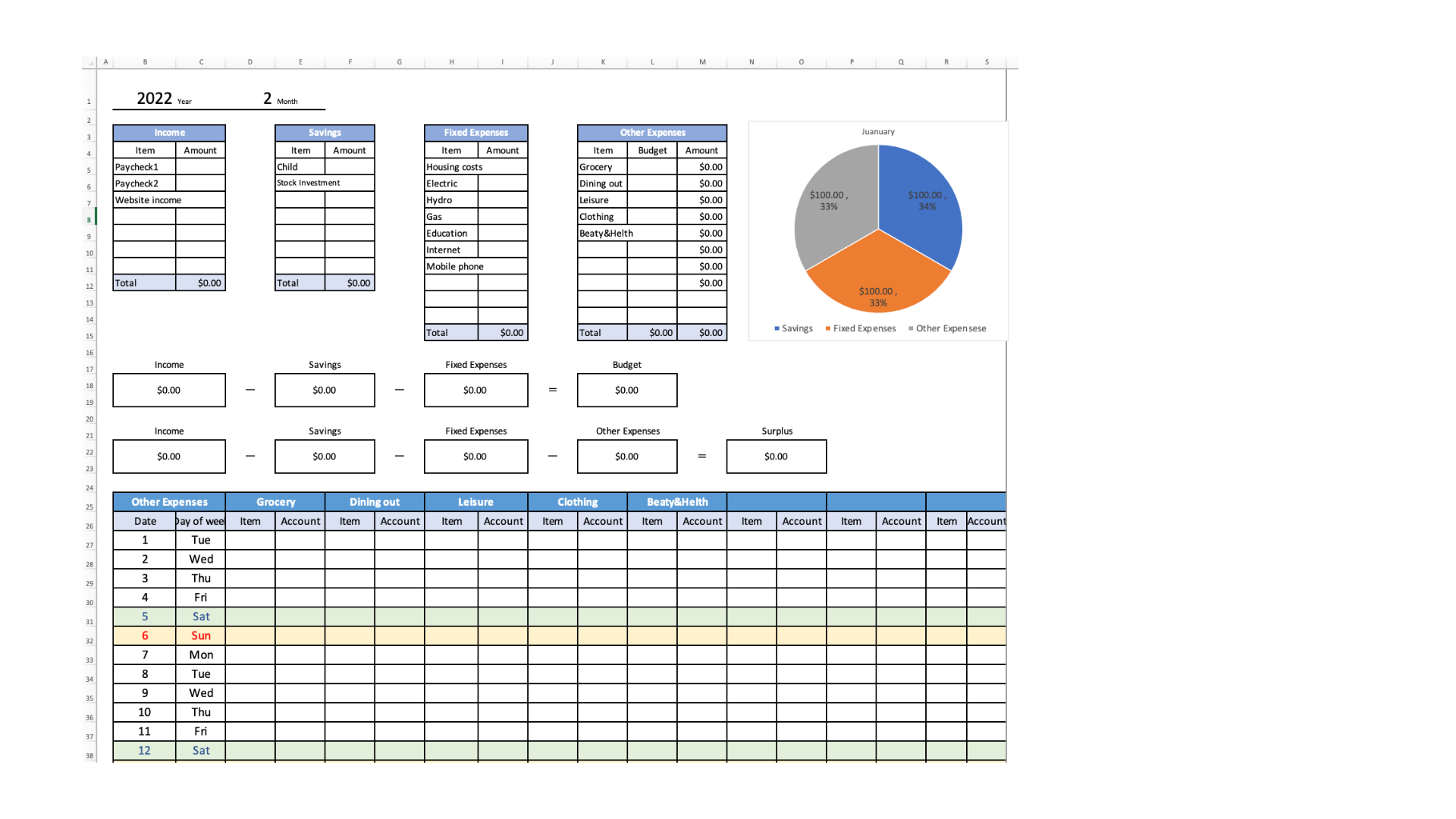
- Categorized into income, savings, fixed costs, and variable costs.
- Income - (savings + fixed expenses) to grasp the monthly budget
- Income - (Savings + Fixed Expenses + Variable Expenses) to figure out the remaining balance at the end of the month
- For variable expenses, categorize them by expense item and date, and enter the item name and amount.
- Use the pie chart to understand the ratio of savings, fixed costs, and variable costs.
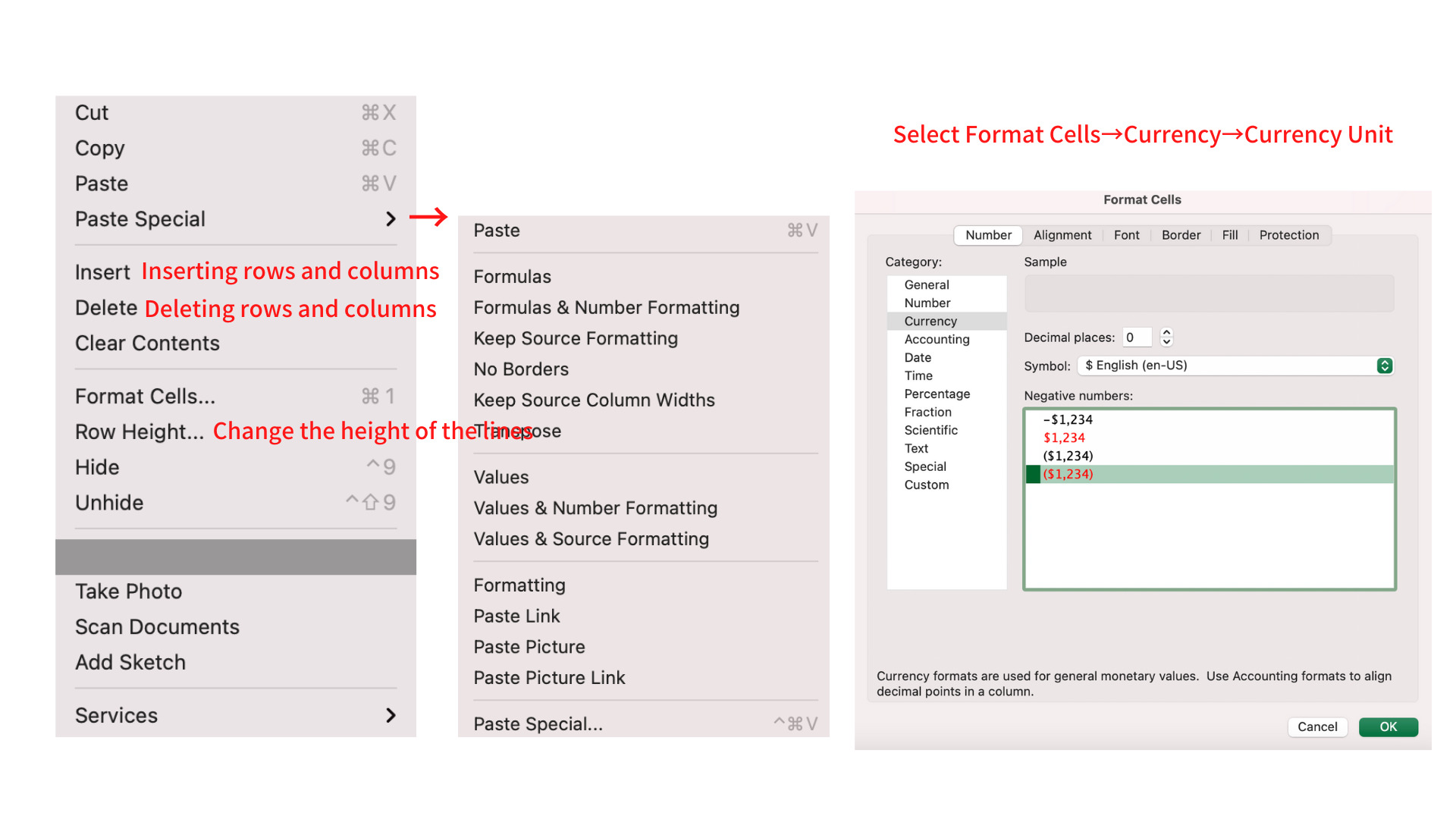
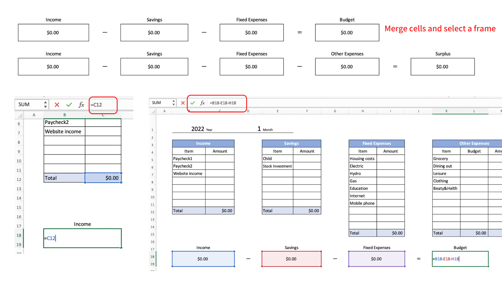
Create a frame for income, savings, fixed costs, and variable costs.
Enter the income, item name, and amount, and enter a formula for the total amount.
In the same way, set up a frame for savings, fixed costs, and variable costs (for variable costs, add a budget item).
Set the monthly budget and the remaining balance
Income - (Savings + Fixed cost) = Budget
Income - (Savings + Fixed Cost + Variable Cost) = Balance
Set the total amount for each in the combined cell.
Rather than copying and pasting, you can display the total amount in a cell like =C11, which saves you the trouble of pasting every time.
Enter a formula like =B17-C23 for the budget and remaining funds.
Entering variable costs
Fill in the beginning date and day of the week, then drag or copy and paste to set the last day.
- Saturdays are shown in blue, and Sundays and holidays are shown in red.
- You can also change the color of the background.
- At the bottom, the total amount is displayed.
Set this total amount to be displayed in the variable cost table above.
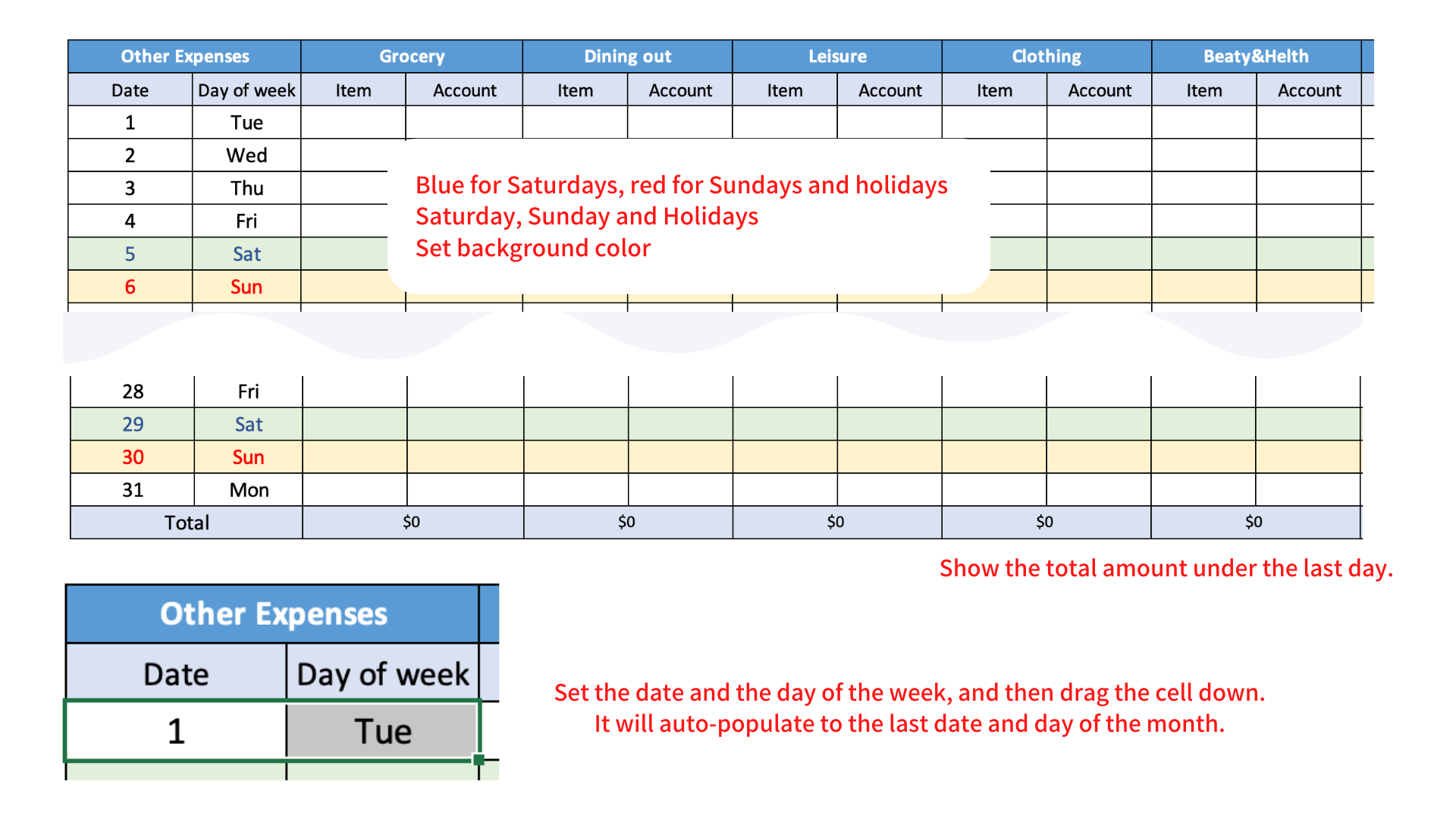
If you want to enter the same expense item more than once in a day, right-click to insert a row.
When you have completed the sheet for the month, copy the sheet to create a new sheet. (For 12 months)
How to set the date (advanced)
So, I'm going to add a feature that is a little more advanced, but can be easily changed using formulas and conditional formatting.
Using this feature, you can change the date, day of the week, text color, and even the background color automatically by simply changing the month portion of January 2022 displayed at the top.
- Enter a formula for the first day's date and day of the week
- Enter a formula for the second and subsequent dates
- Get the WEEKDAY
- Change the text color of Saturday and Sunday by conditional formatting
- Set holidays and change text color by conditional formatting
- Change the background color of weekends and holidays with conditional formatting
Date and Day Setting
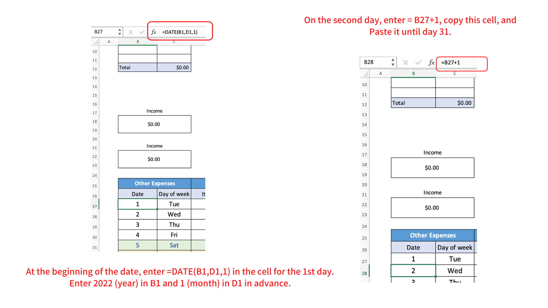
Enter =DATE(B1,D1,1) in the cell for the first day, date 1.
Enter the year and month in B1 and D1 in advance. (The top part of the completed image)
If you want to change the beginning date to match your payday, etc., enter the desired date in the last 1.
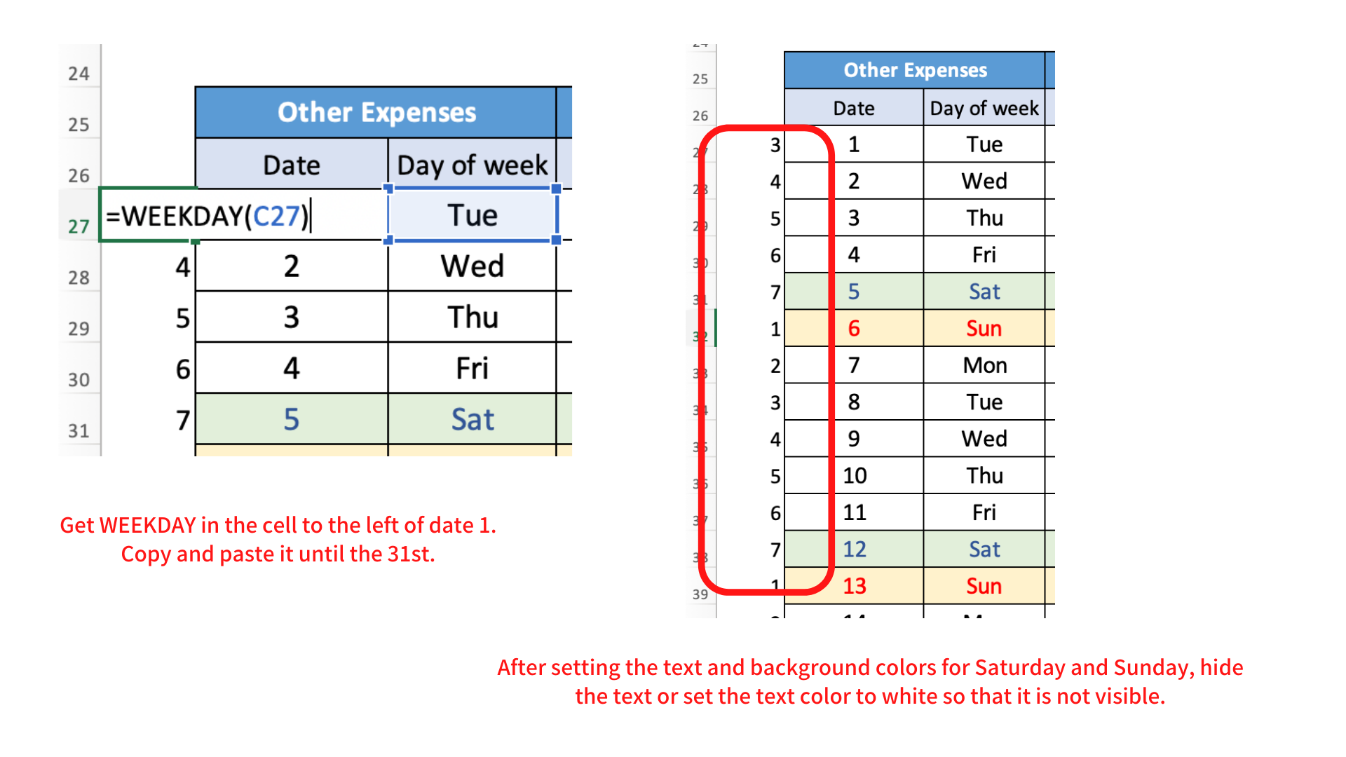
On the second day, enter =B27+1. (The day of the week with 1 added to the cell for day 1)
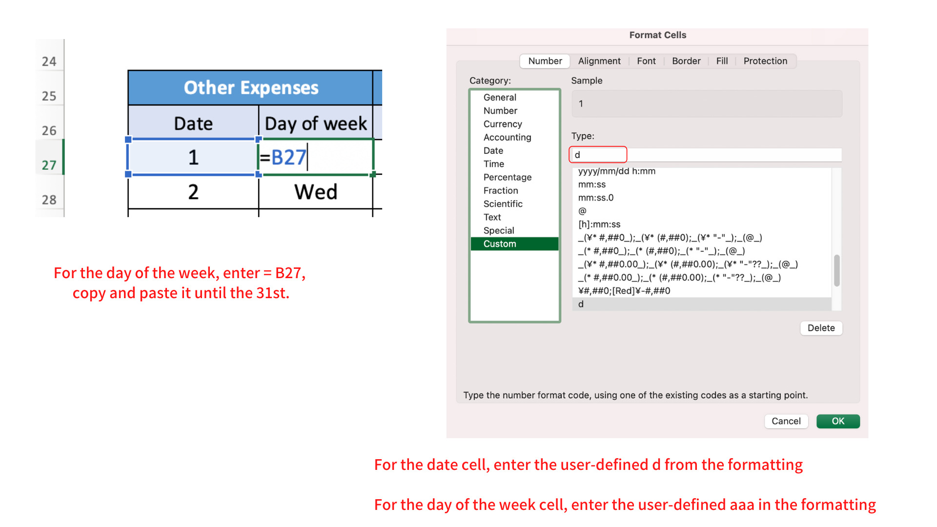
For the day of the week, enter =B27. (= the cell in which the next day is entered)
For the date, copy the cell for day 2 and paste it to day 31.
For the day of the week, copy the first cell and paste it until the 31st day.
In the cell formatting, select the date cell and type user-defined d.
Select the cell for the day of the week, and type user-defined aaa.
Changing the text color for Saturday and Sunday
To determine the cells for Saturday and Sunday, get the WEEKDAY.
Enter = WEEKDAY(C27) in the cell to the left of the first day's date. (= WEEKDAY(date) to display the day of the week from 1 to 7)
Copy the cell and paste it until the 31st day.
(= WEEKDAY (date) to display the days of the week from 1 to 7.
After setting the text color and background color for Saturday and Sunday, hide or set the text color to white so that the WEEKDAY indicator is not visible.
To hide the text, select a row, right-click, and click "Hide".
Saturday will be displayed as 7 and Sunday as 1.
Set the conditional formatting so that column A is blue when the value is 7 and red when the value is 1.
Select the date and day range (B27 to C57) and click on "Conditional Formatting" on the home screen.
Click on "New Rule" and then "Use a formula to determine which cells to format".
In the formula field, enter =$A27=7.
(When the value after A27 in column A, where WEEKDAY is entered, is 7 (Saturday))
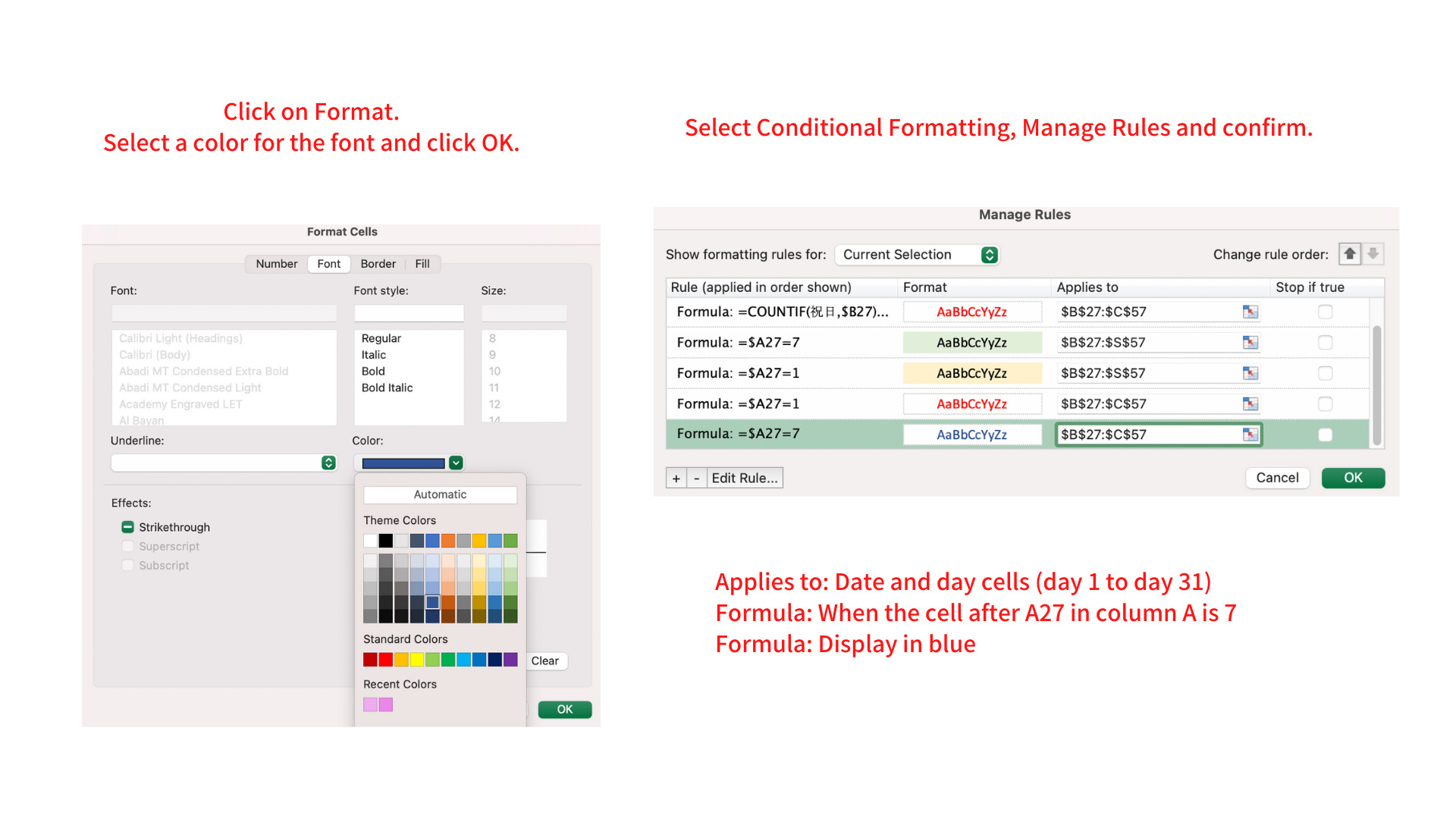
Click on the format and select blue.
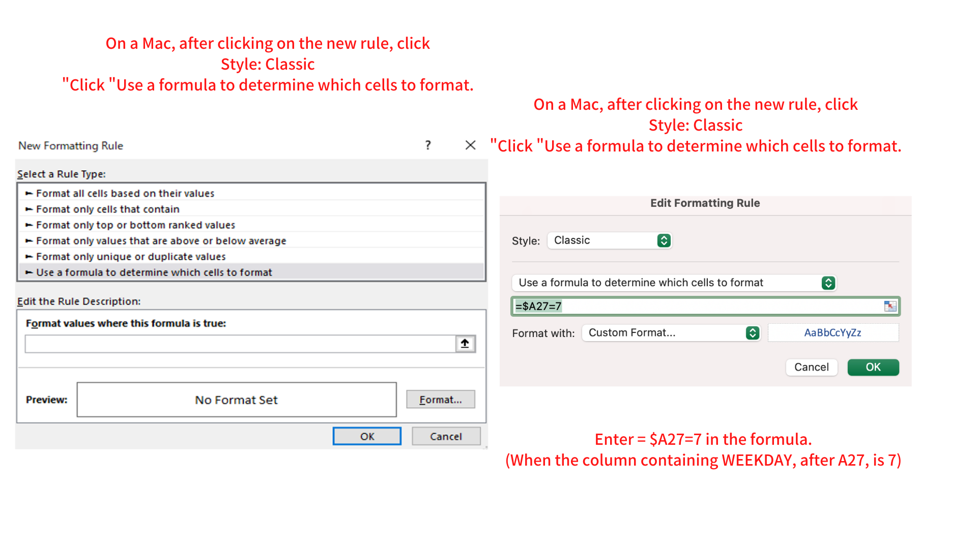
Check what you have entered from the Manage Conditional Formatting Rules section of the home screen.
Apply to: the selected range (the range you want to display in blue)
Formula: =$A27=7
Format: Blue
Set Sunday in the same way.
Formula: =$A27=1
Format: red
Setting holidays and changing text color
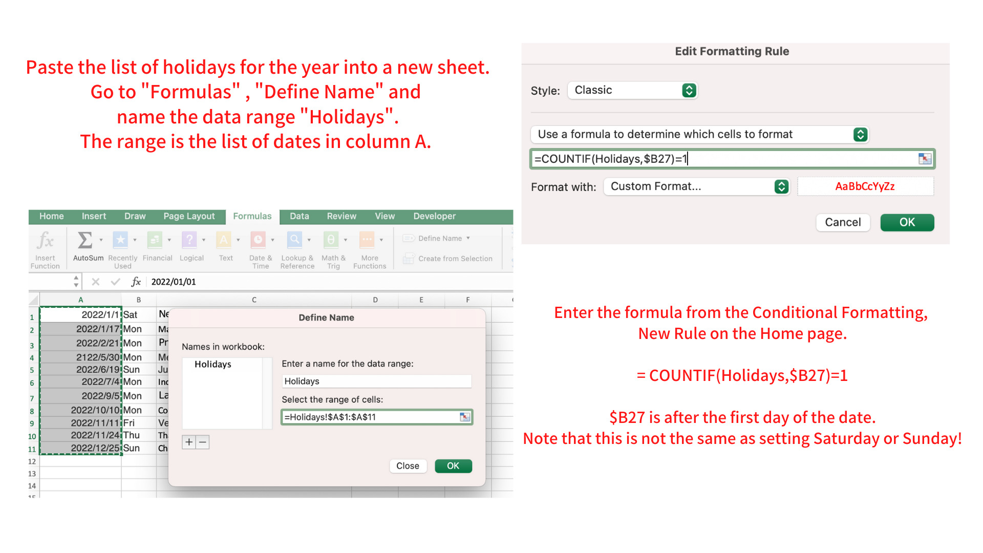
Find the list of holidays for the year and paste the dates into a new sheet.
Select the list of dates only, and name it "Holidays" by clicking on the formula name definition.
Go back to the month sheet of the Household Budget and select a range of dates and days.
Set the formula from the new rule for conditional formatting and change the format to red.
= COUNTIF(Holidays,$B27)=1
The $B27 determines if there is a holiday in the date after the first day of the date column.
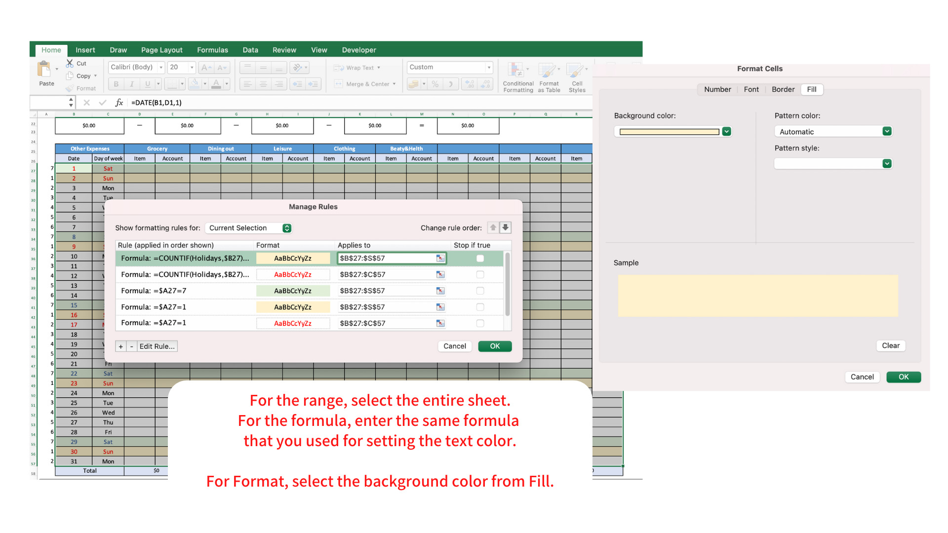
Changing the background color of weekends and holidays
We want to change the background color of the day of the week column, so for the range, select the entire sheet.
Set the formula and background color from the new rule for conditional formatting.
For the formula, enter the same formula that you used for setting the text color.
For the formula, set the background color of the fill to a color of your choice.
Create a month sheet by purpose
In this example, we will set up a household budget for two purposes: to save money on food and to reduce wasteful spending.
Saving money on food
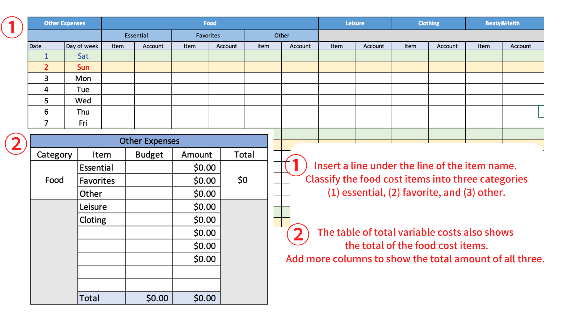
As an example of saving money on food, if you want to cut down on luxury items (alcohol, sweets, etc.),
You can categorize your food expenses into (1) essential, (2) luxury items, and (3) others to know how much luxury items you are consuming in a month.
(1) Add a line to the variable cost item column and classify the food cost items into three categories.
2) Add a column for total food cost to the table of total variable cost.
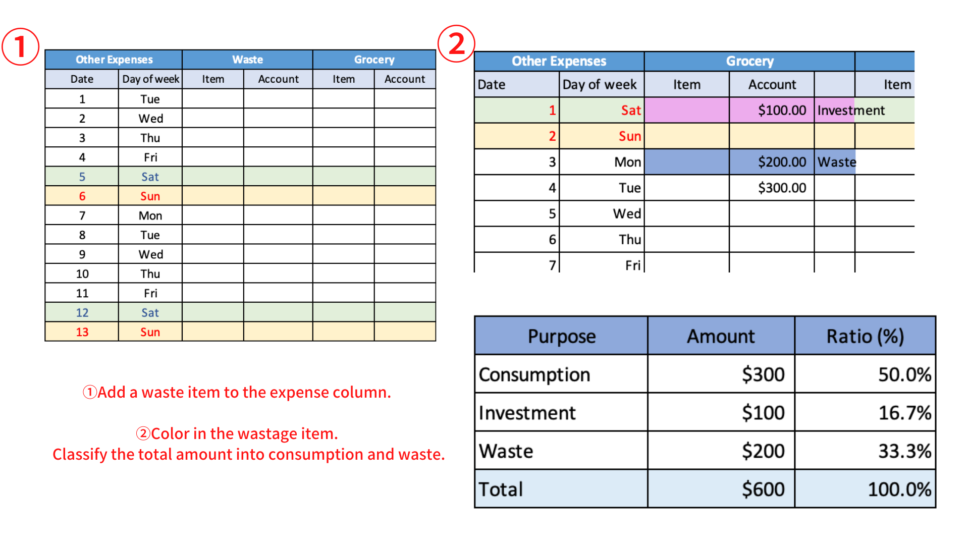
Reducing Wasteful Spending
In order to reduce wasteful spending, you need to find out how much you are wasting each month.
- Add a waste item to the expense column to show the amount of money you have wasted.
- Color the items and amounts of wasteful spending, and display the total amount at the end of the month.
If you want to color in the wasted money, it will be difficult to calculate the total amount if you use the method of coloring in each time.
So we'll use a regulated list, conditional formatting, and formulas to automatically color and display the total amount when we select "Waste".
Add a column to the right of the amount column.
Select the cell where you want the list to appear.
Click on "Input Restrictions" for data and select "List".
In the original value column, enter "Waste" (If you want to add an investment item as well, enter "Waste, Investment".
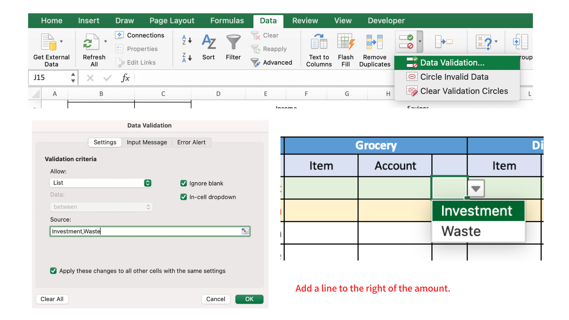
In the conditional formatting, set the background color to change when waste and investment are selected.
Select the range where you want to change the color.
Click on Home Screen, Conditional Formatting, New Rule, Use Formula to Determine Cells to Format.
Enter =$J15="Waste" in the formula
(When the cell after J15 in column J is displayed as "Waste".)
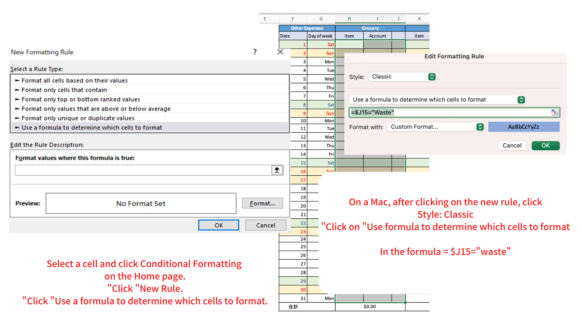
Select your favorite color from Format Cells, Background Color, and Fill, and click OK.
Similarly, set the color for "Investment" using conditional formatting.
When you click on the cell you have set, a pulldown will appear. Make sure the color changes when you click on Waste or Investment.
If you want to modify it, you can check and edit it from the conditional formatting rule settings.
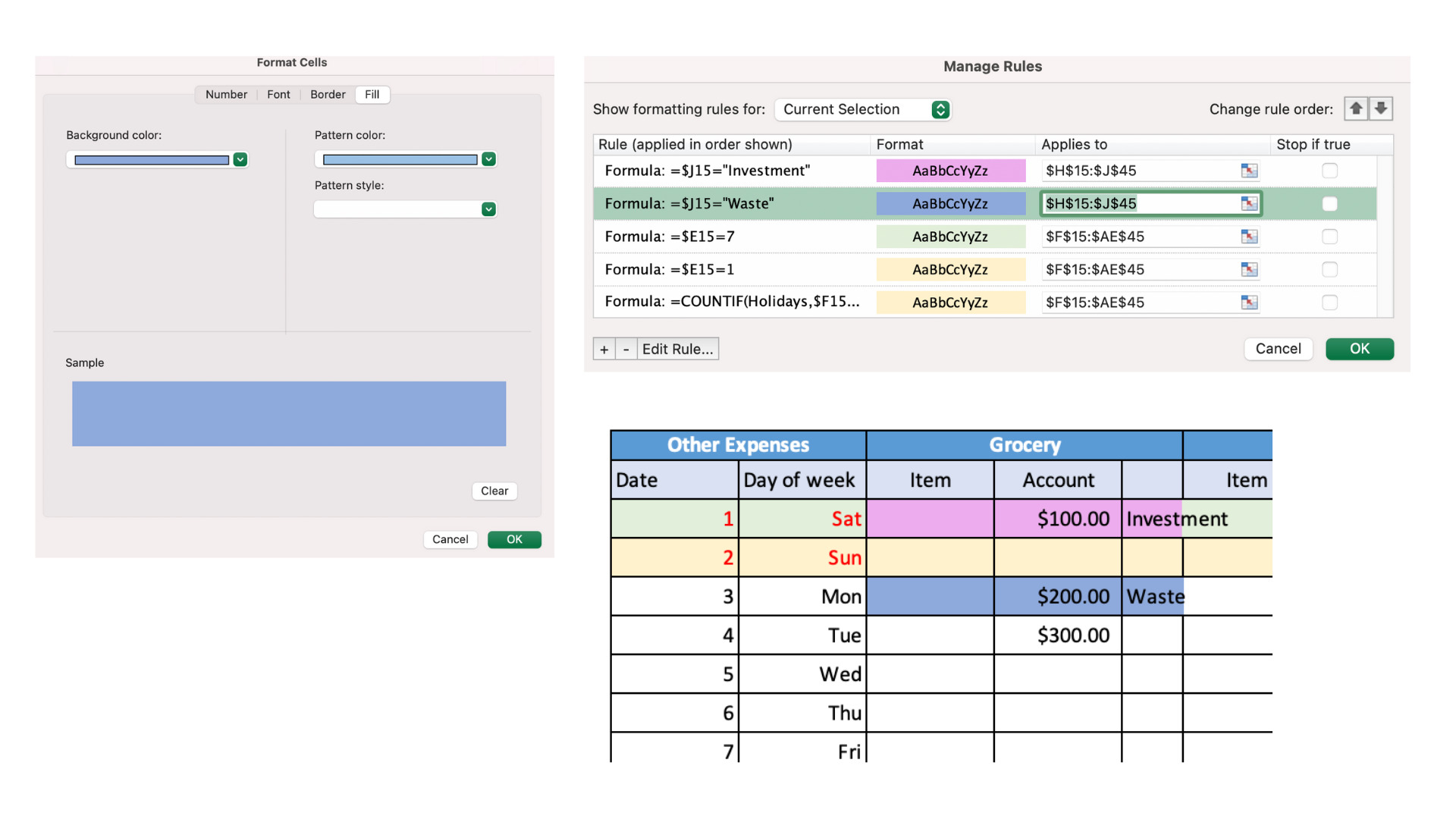
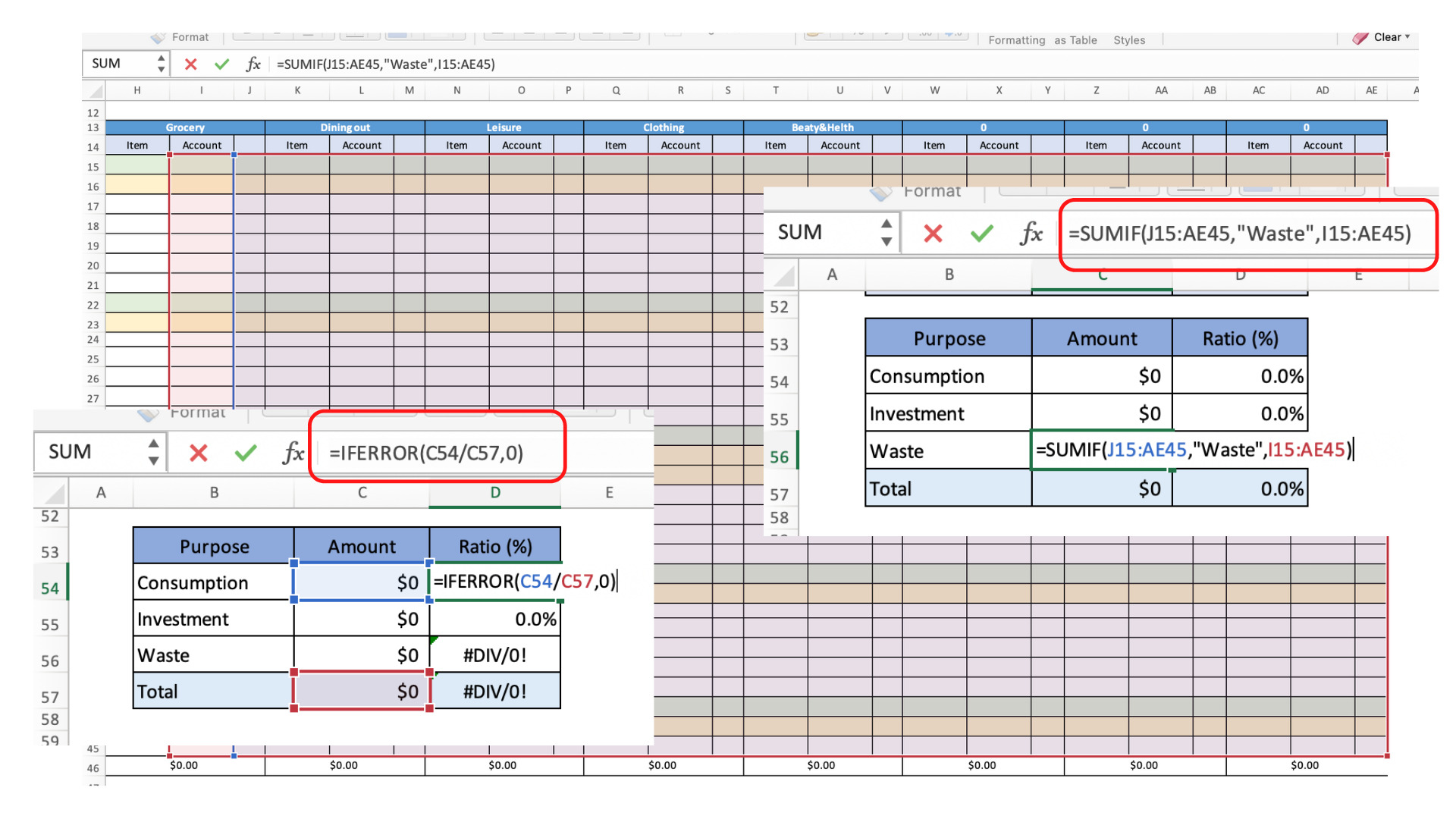
In the same sheet, create a table to display the amounts and percentages of consumption, waste, and investment.
Use the SUMIF function to display the total amount for waste and investment.
In the amount of waste cell =SUMIF(J15:AE45, "Waste",I15:AE45)
In the amount of investment cell =SUMIF(J15:AE45, "Investment",I15:AE45)
In the total amount cell, display the total amount of variable expenses.
In the consumption amount cell, enter =total amount-(waste amount + investment amount).
For the ratio, enter consumption / total amount =C54/C57, and right-click on the cell and change the unit to percentage.
In this case, if no amount has been entered, it will show #DIV/0!
If you are concerned about this, type =IFERROR(C54/C57,0) to display 0, or =IFERROR(C54/C57,"") to leave it blank.
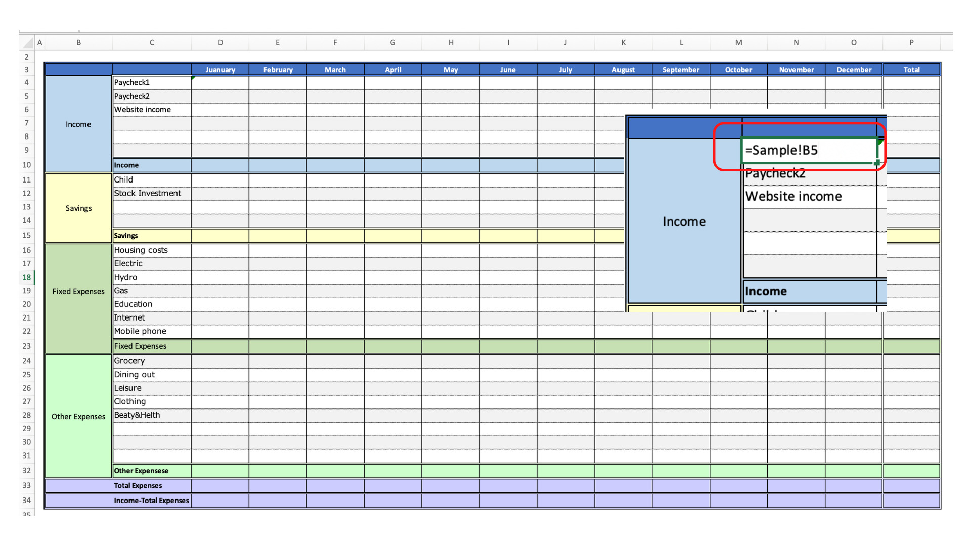
Annual Transition Table
Create an annual trend table on a new sheet.
The vertical axis shows income, savings, fixed expenses, variable expenses, total expenses, and income minus expenses.
On the horizontal axis, display January through December and the annual total.
Each value can be copied and pasted each time, or values from other sheets can be displayed, as in =Sample!C5.
For total expenses, use the SUM function to set total savings, total fixed expenses, and total variable expenses.
For income-expenses, enter =total income-total expenses.
Create a graph
Create a graph of the transition table
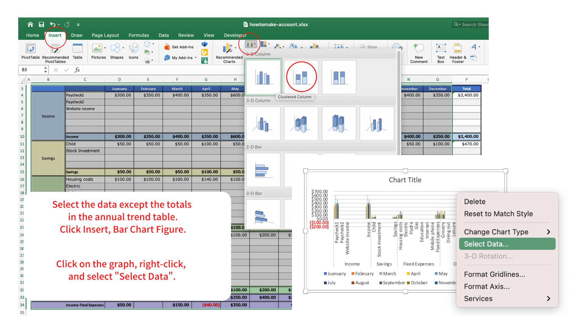
Select all the data in the yearly transition table, and select Insert, Bar Chart.
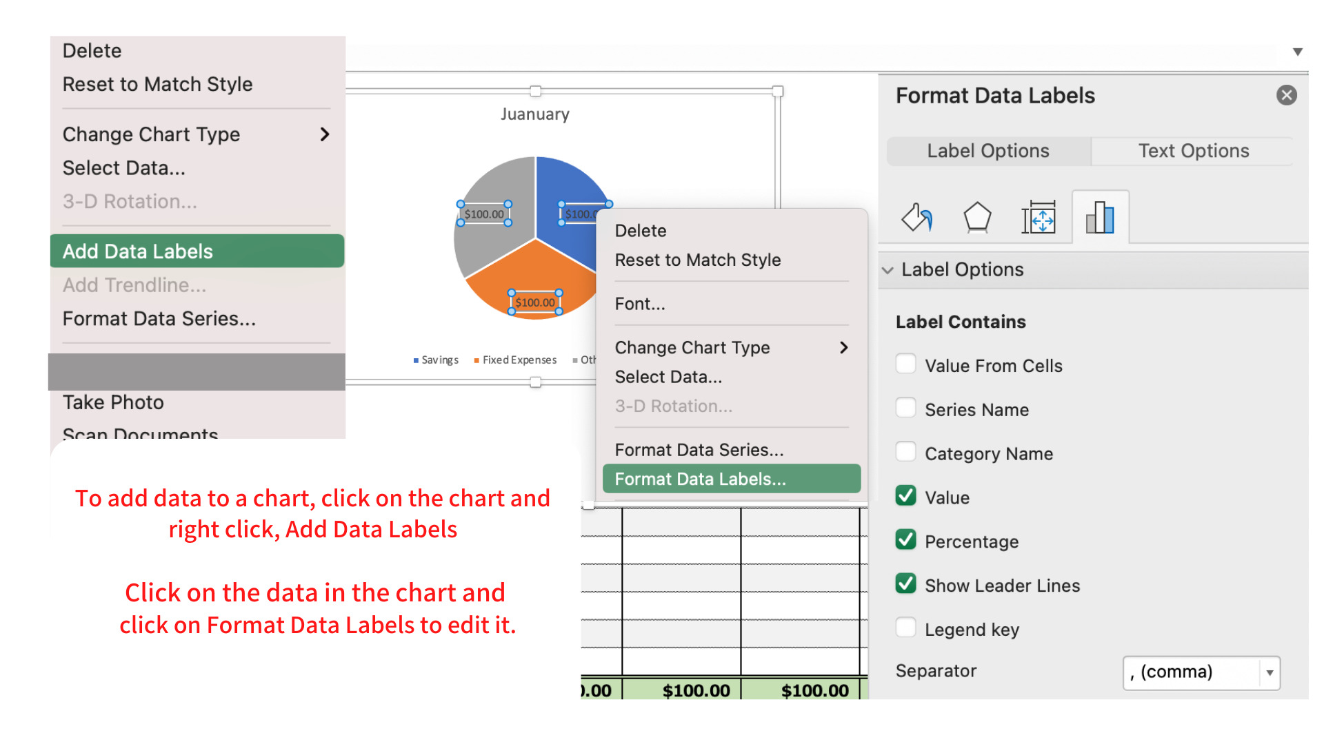
To modify the graph, right-click and select "Select Data".
Click "Toggle Rows/Columns (W)" and uncheck the data you do not want to display, leaving the checkboxes for the data you do want to display.
For the horizontal axis label, select January through December.
For the vertical axis, select Total Income, Total Savings, Total Fixed Expenses, and Total Variable Expenses.
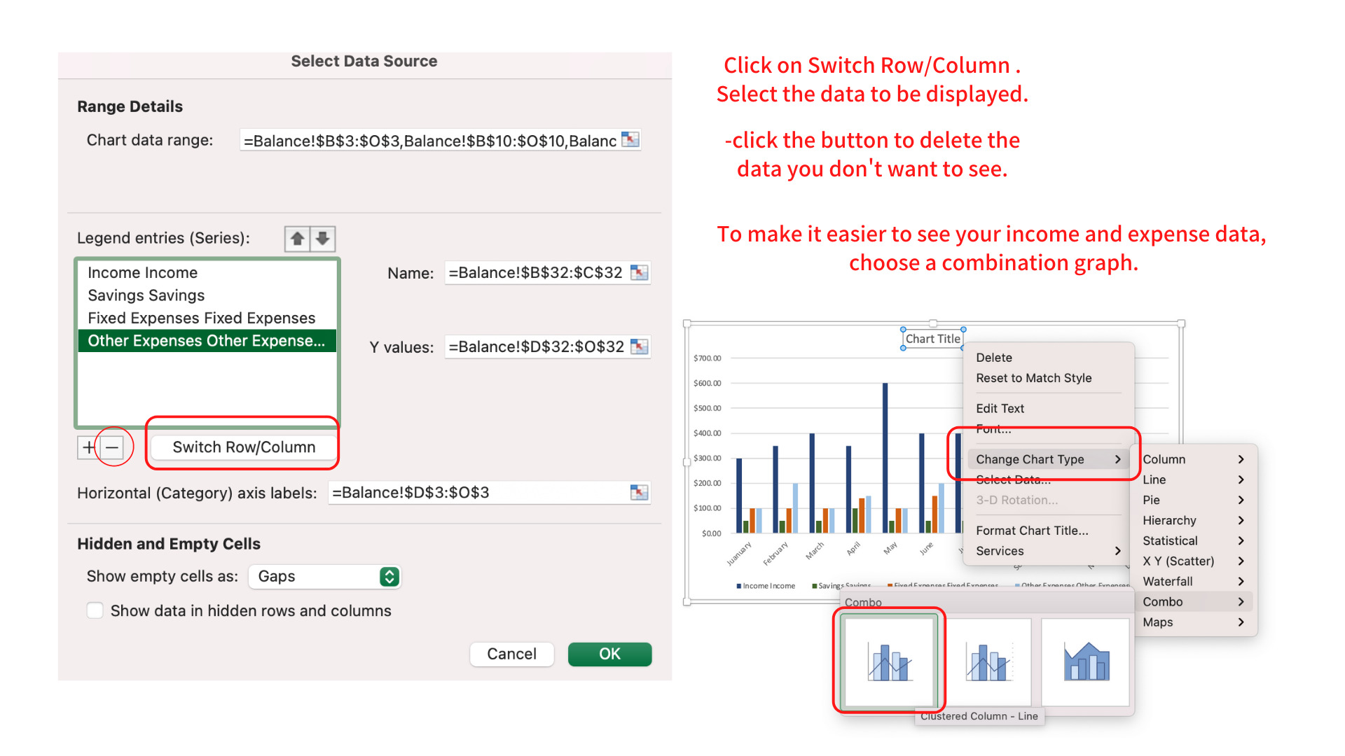
To categorize income and expenses, change the graph type.
Select a graph, right-click, and select Change Graph Type.
Click "Combine" and select Line Chart for income and Stack Chart for expenses.
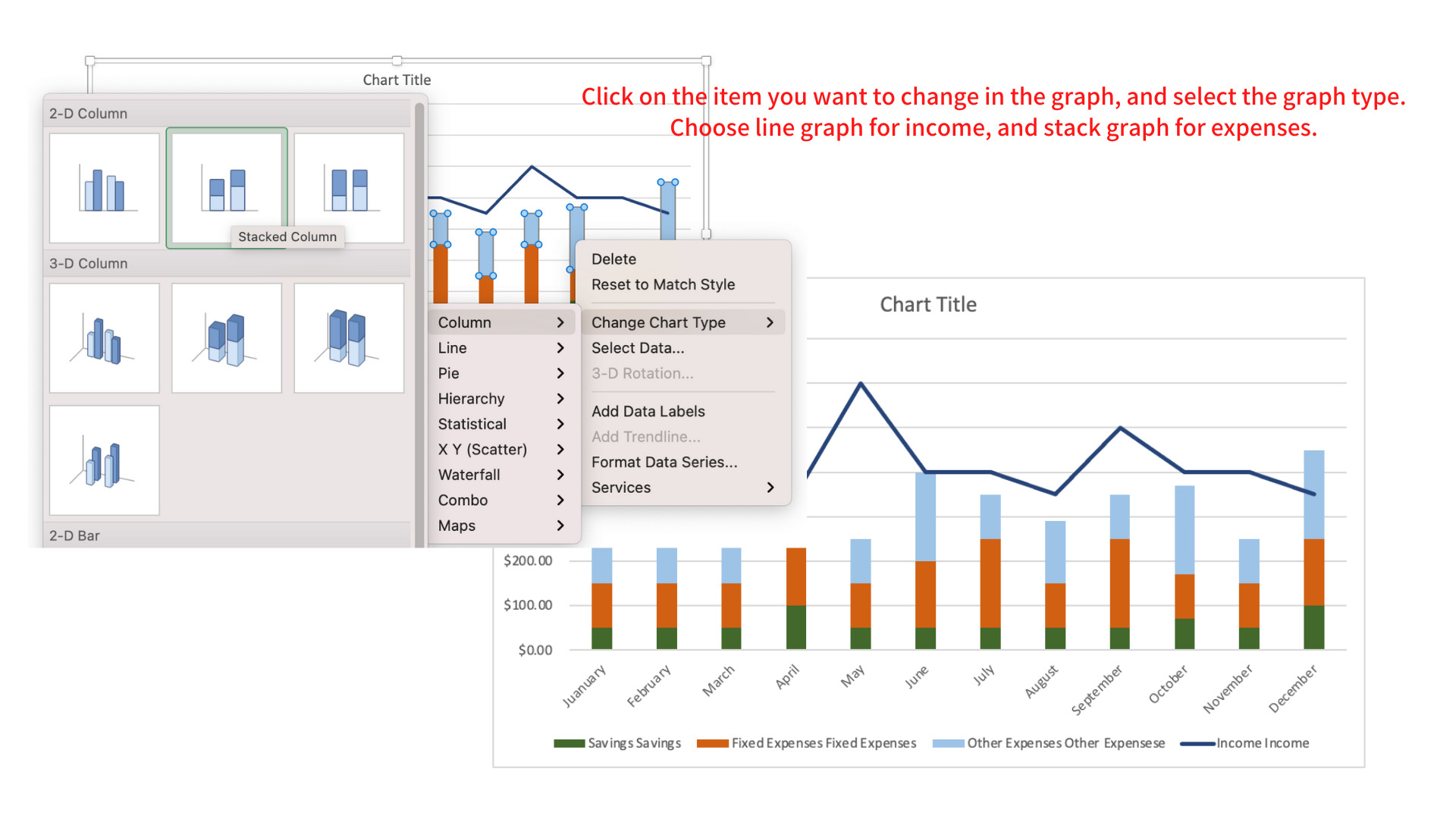
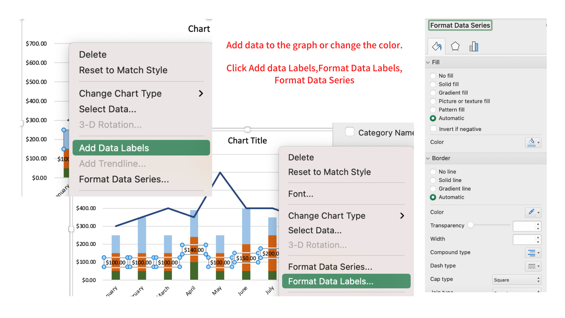
To change the format and color of the graph, right-click and select Format Data Series.
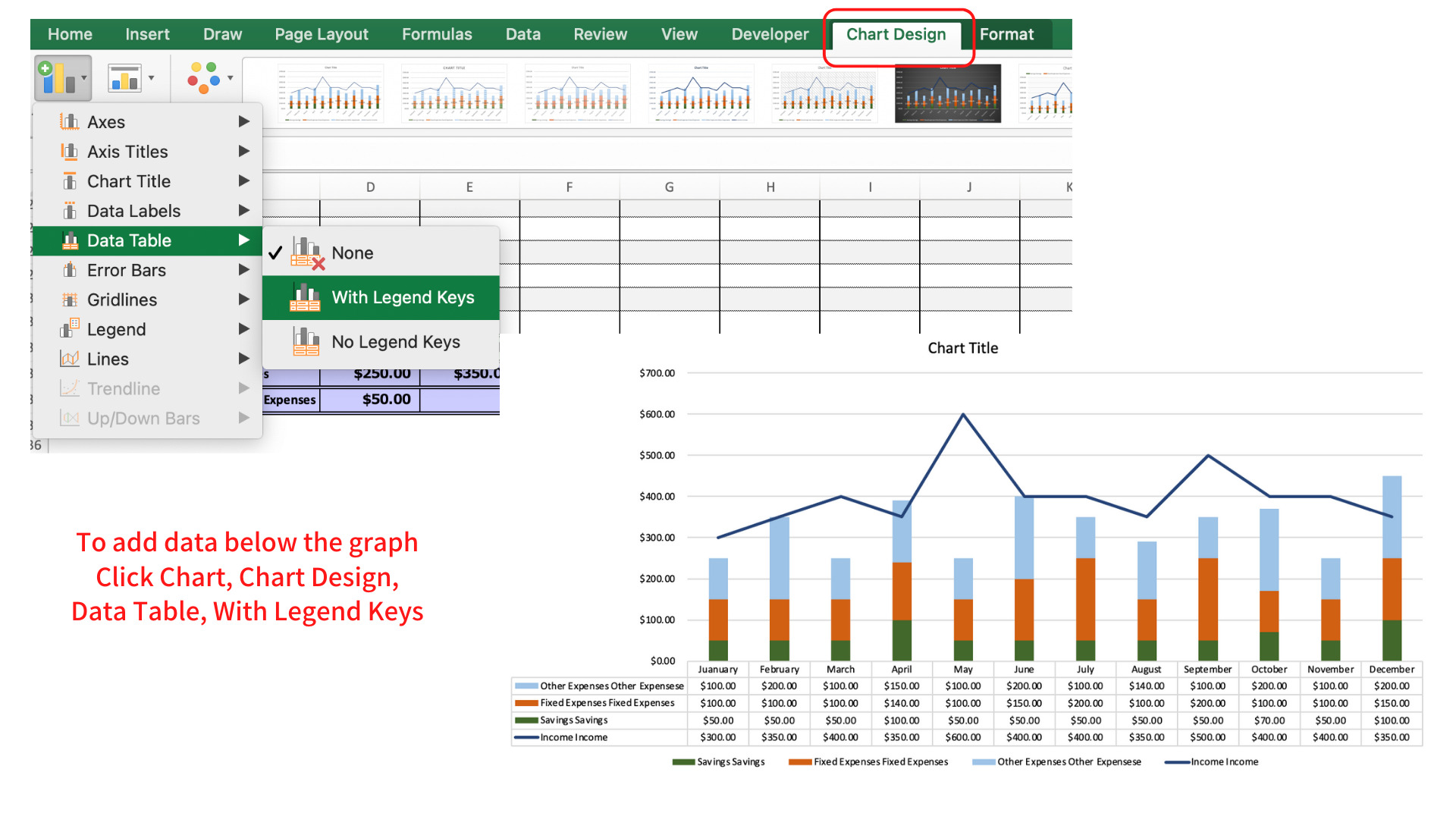
Click the Chart Design and select Data Table to display the data below the graph.
Create a monthly pie chart
To create a pie chart, the data will be created using the data from the transition table.
As with the trend chart, select the data, click Insert, and select the pie chart symbol.
When the pie chart appears, select the graph, right click, and click Select Data.
Leave the checkmarks for the data you want to display, and uncheck the checkmarks for the data you do not want to display.
For example, select D15, D23, and D32 for the Y values.
For Horizontal axis labels, select C15, C23, C32.
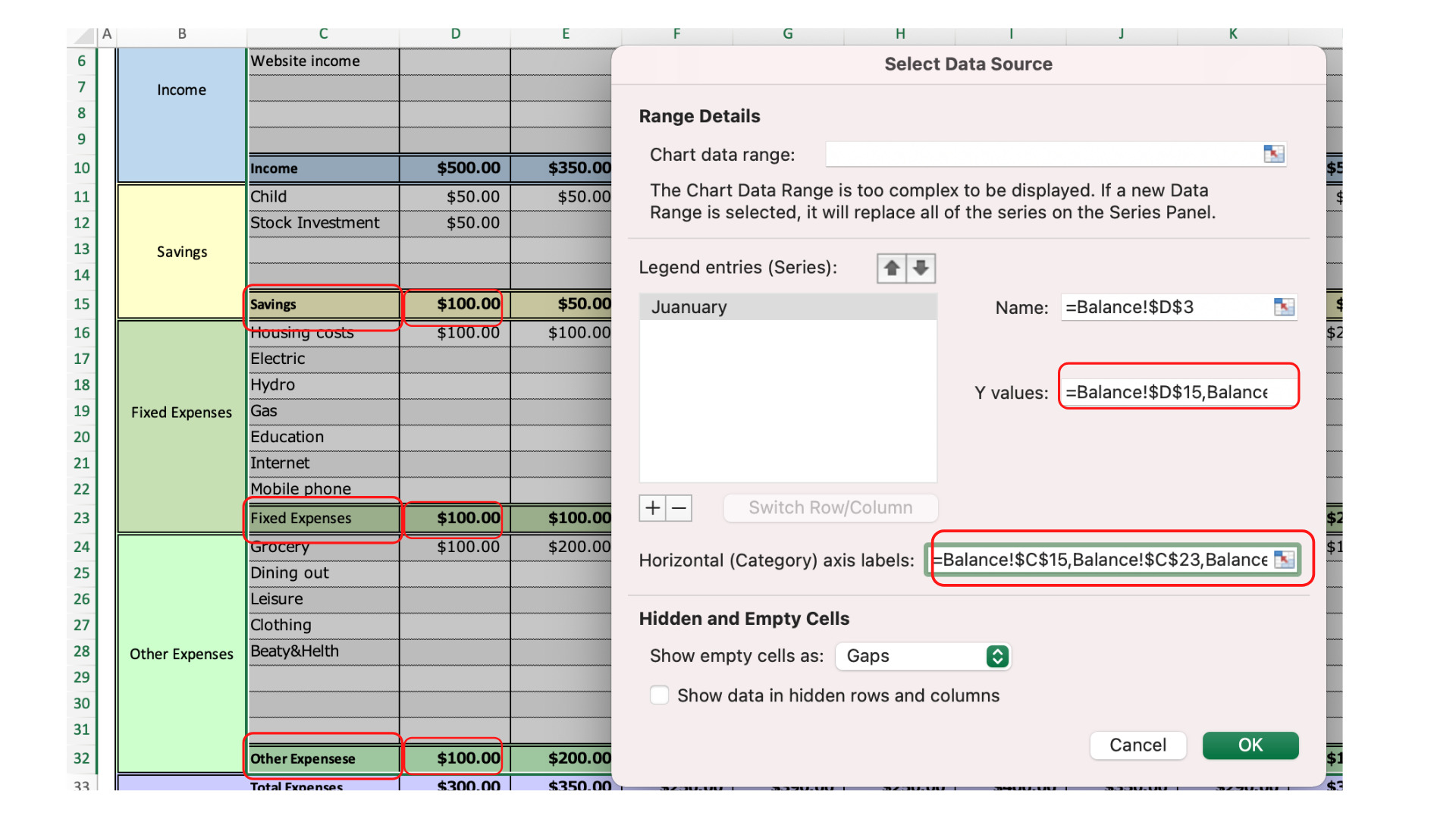
The legend item is January (select the month you want to create the graph).
For the horizontal axis labels, select Total Variable Costs, Total Fixed Costs, and Total Savings.
To print and use
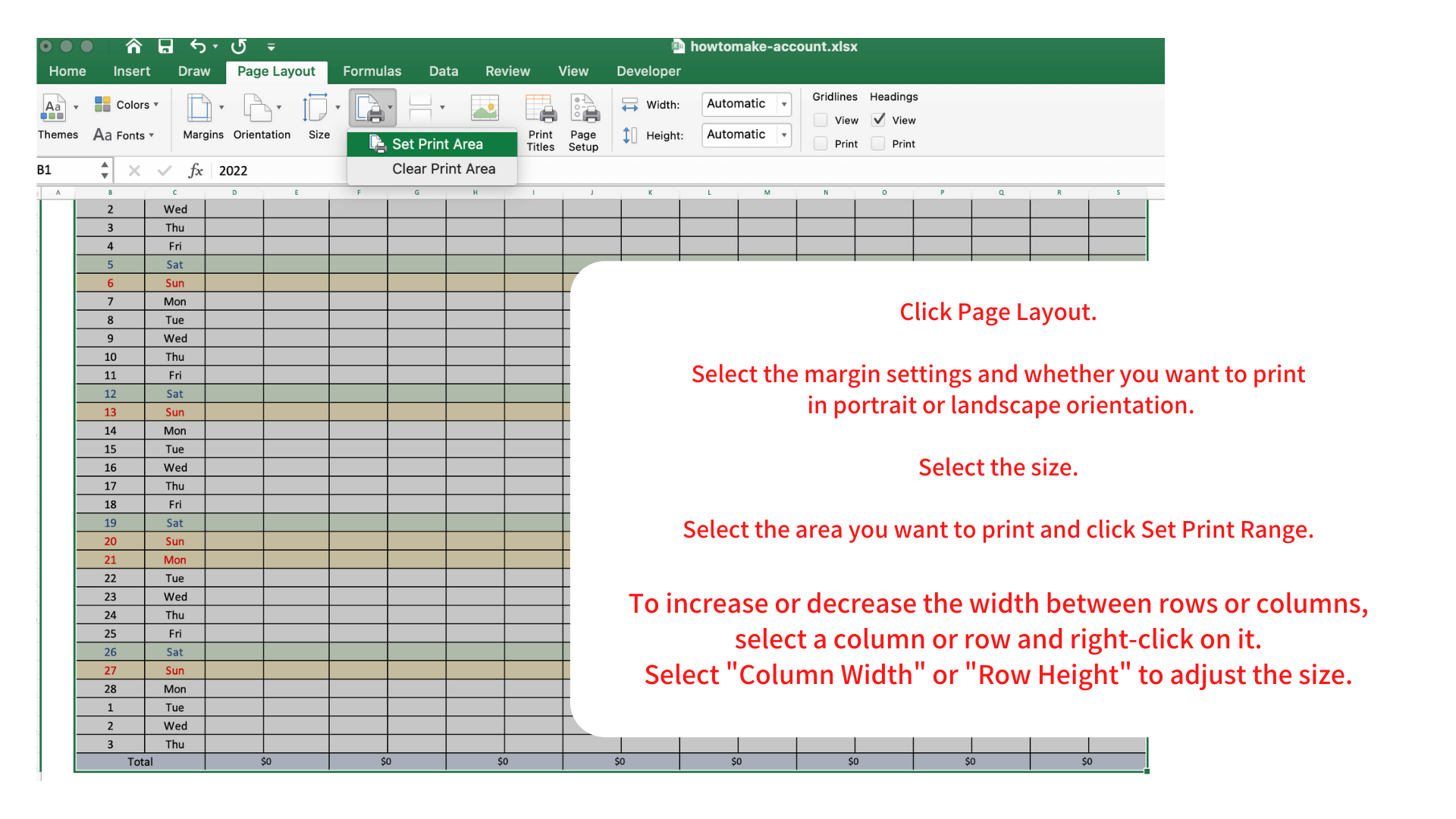
Click Page Layout.
Adjust the margins, select the print orientation (portrait or landscape), select the paper size, and click "Print".
Select the area to be printed, and click Print Range Settings.
If you want to adjust the row spacing or column width, select a row or column, right click, select "Column Width" or "Row Height" and adjust the size.
If there are any formulas in the cells and they are displayed as (e.g. the total amount), please make sure that they are not visible before printing by changing the text color to white.
Sample Download
You can download the sample sheets explained in the How to Make an Excel Family Budget for free.
The sample includes a monthly sheet, a sheet for each purpose (saving money on food, reducing wasteful spending), an annual chart, and a graph.
Click on the download button to download the Excel file.