How to create a kakeibo in a spreadsheet

I don't know how to make a kakeibo in a spreadsheet.

Do you have such a problem?

Although spreadsheets and Excel look similar, there are some limitations such as functions that can be used in Excel cannot be used in spreadsheets.

Instead of giving up because of the limitations, I will show you how to create a kakeibo that has the same functions as Excel using other formulas.

This kakeibo uses a pivot table that can aggregate and analyze large amounts of data.

It is recommended for those who want to analyze the data thoroughly, as it can be analyzed from various perspectives, such as by expense item, by account, or by store.

Features of this kakeibo

• Enter expense, account, and store names on the setup sheet
• Record daily household accounts on the input sheet
• Compare monthly household accounts on the Annual sheet
• Pick up only the information you want to know by expense, account, store, etc.

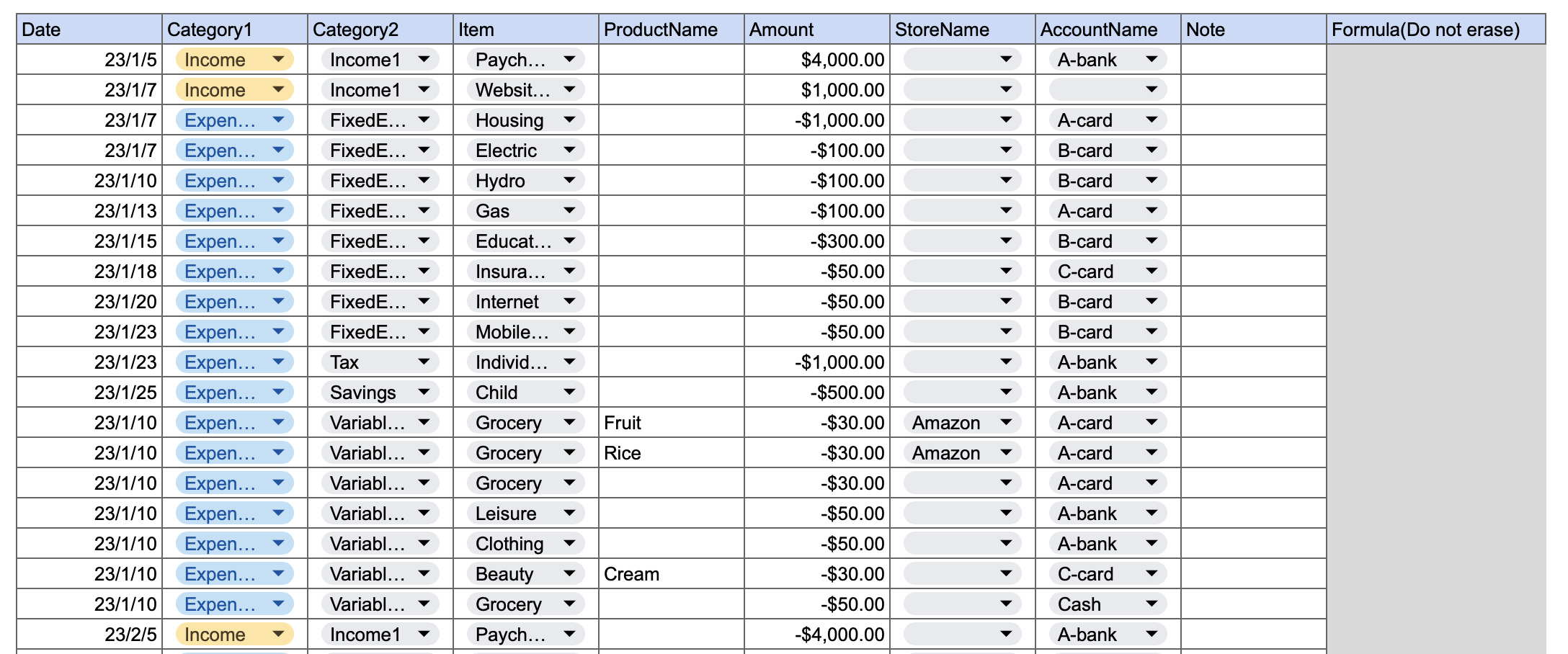
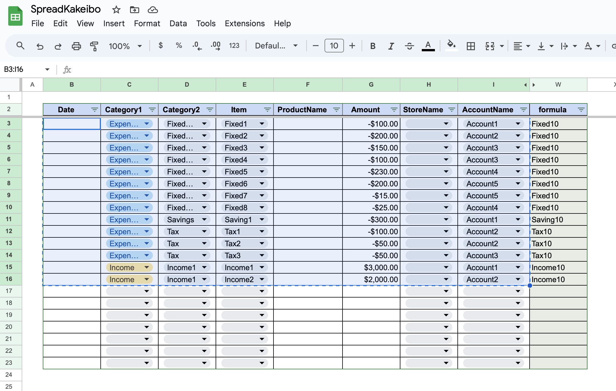
Input sheet

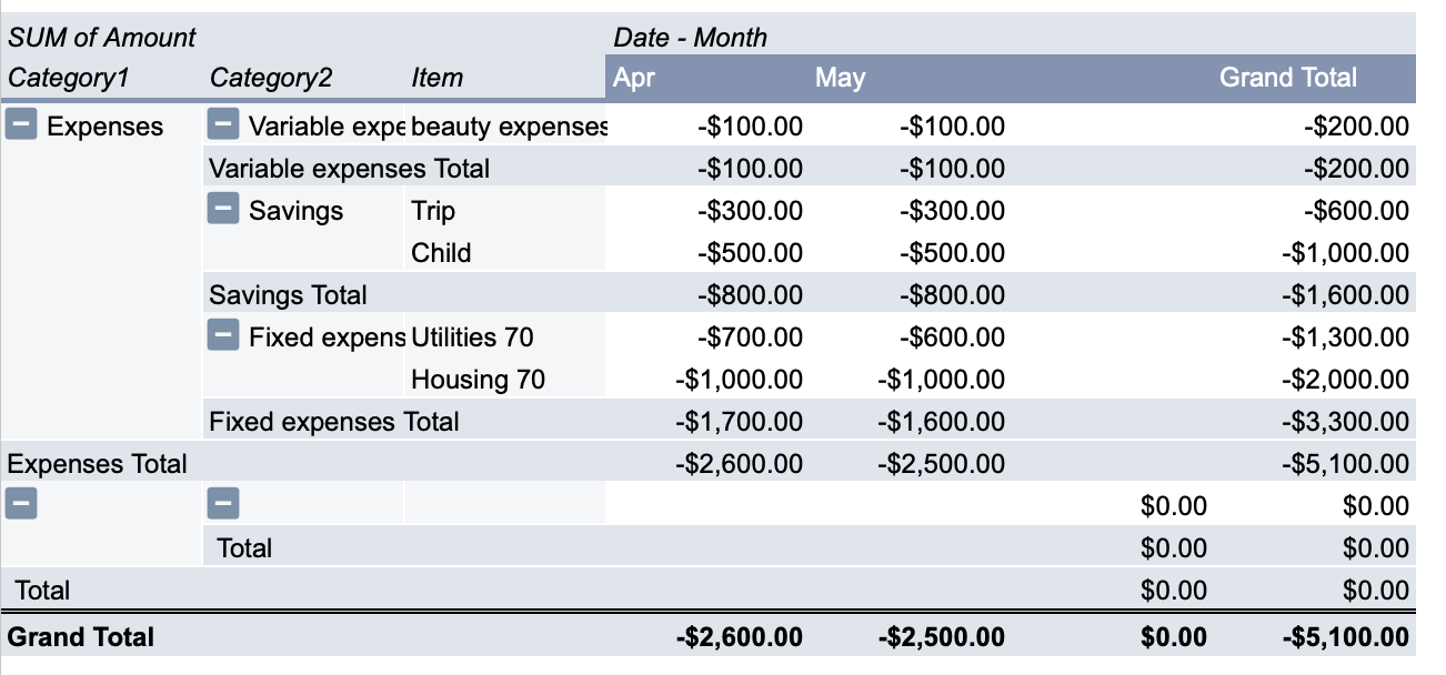
Pivot table

How to Create a Household Budget Book

Create New File

Open the Google Spreadsheet page.

You will need an account to use the spreadsheet.
If you do not have one yet, please create a new one before use.

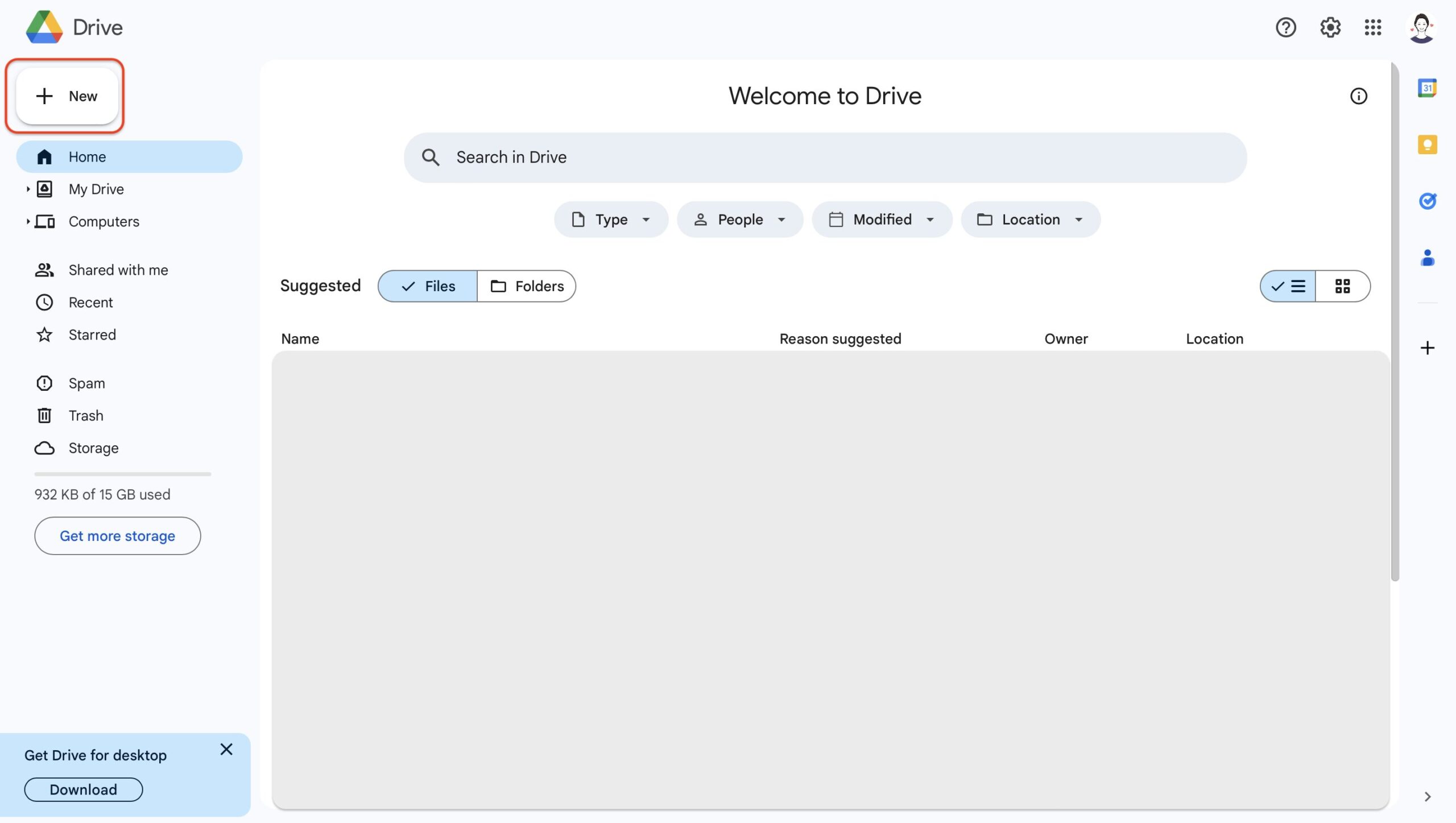
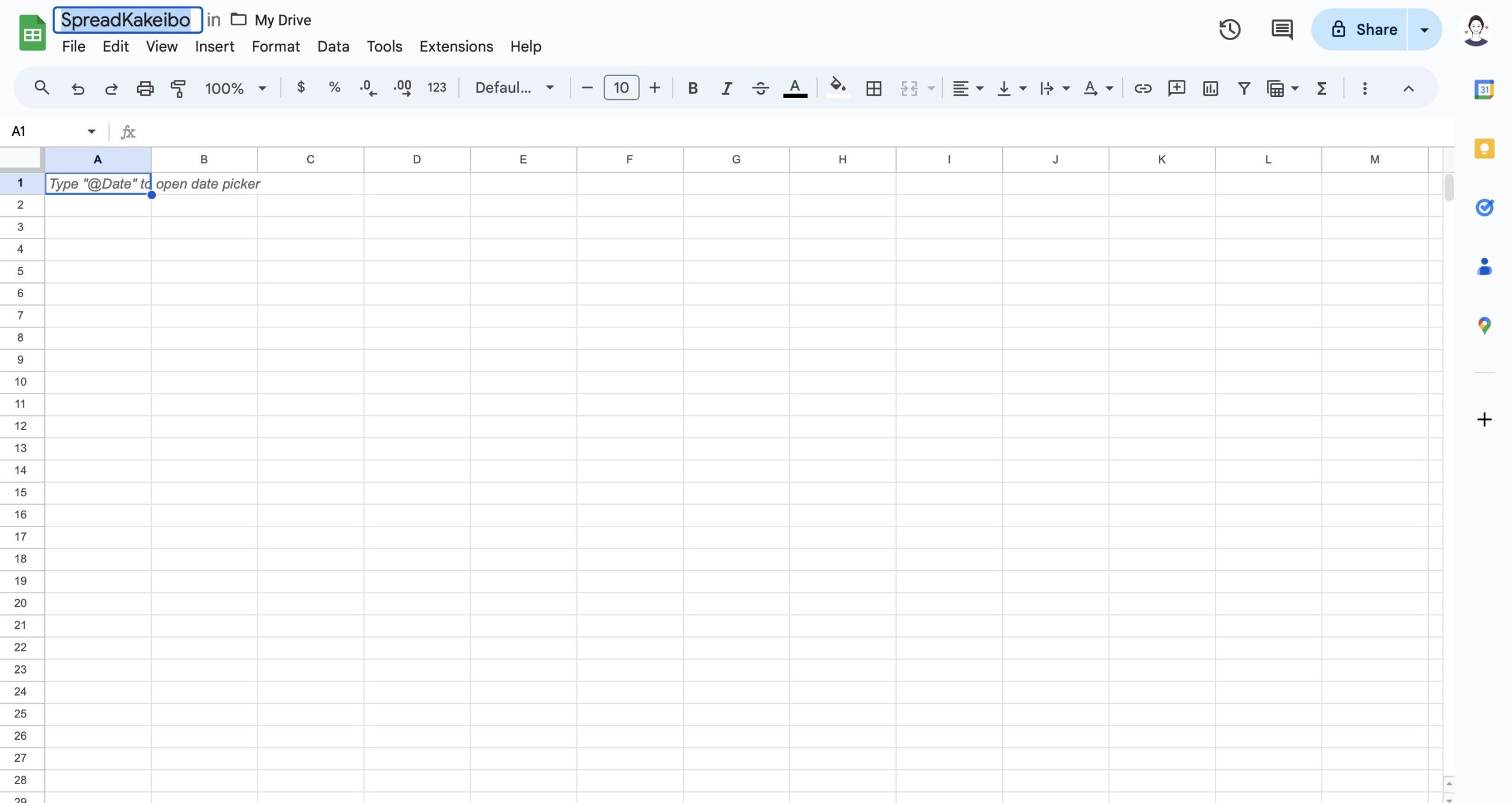
After logging into the spreadsheet, click on "Blank Spreadsheet".

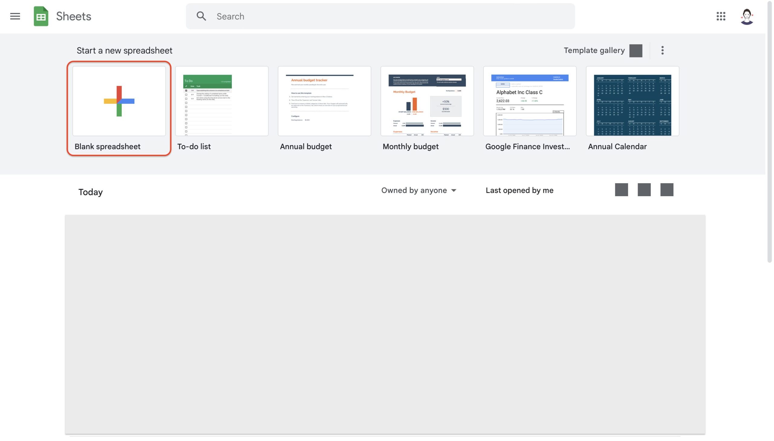
Name the spreadsheet.

Setup Sheet

What to do first

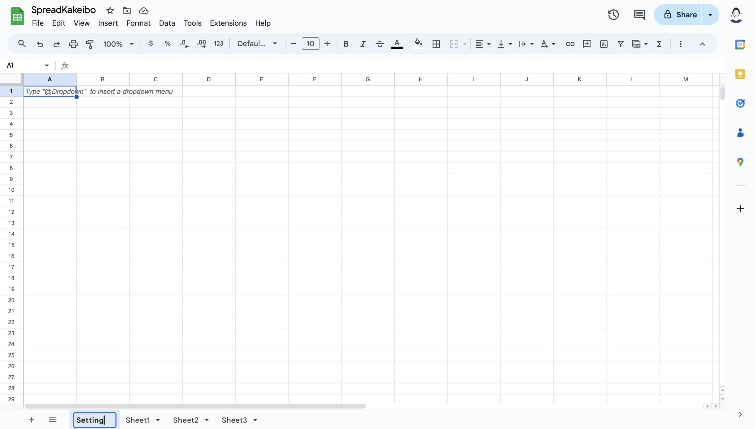
Click the + button in the lower left corner to add a sheet.
Change the sheet name to "Setting".

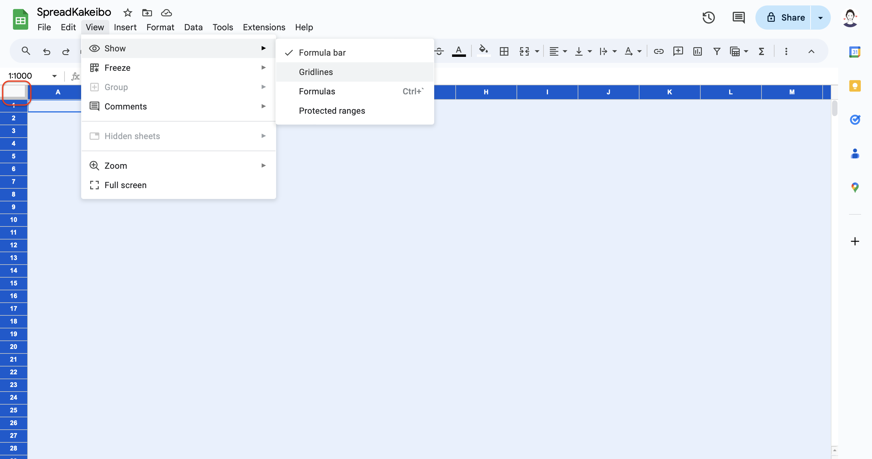
To make the table easier to read, remove the grid lines.

Click on the top left square and select all ranges.
Uncheck the Gridlines in the "View".

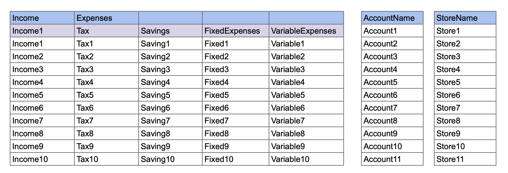
Set up Item

• Income
• Taxes
• Savings
• Fixed Expenses
• Variable expenses
• Account
• Store Name

Be sure to enter "Income 1" on the line below Income.

This is required for the setup on the input sheet.

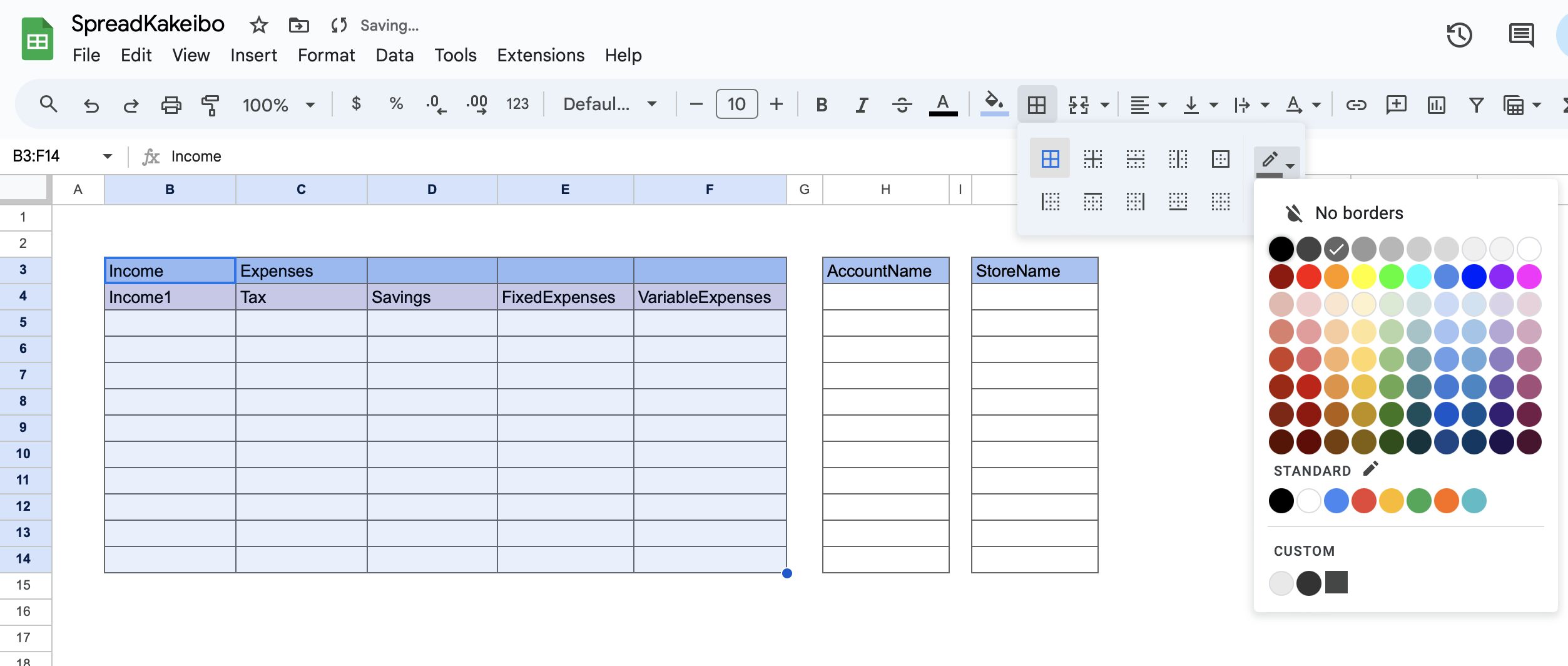
Set the framework

Select the area to be bordered and click on the table symbol in the menu bar.

Select the type of table and the type of line.

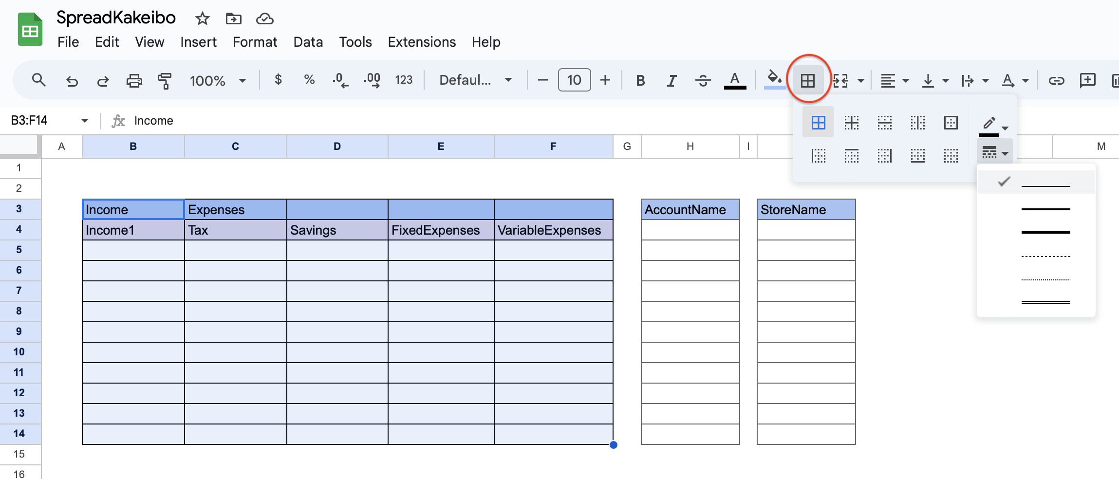
Change the color of the line.

Set background color

Select the area for which you want to change the background color and choose the fill symbol.

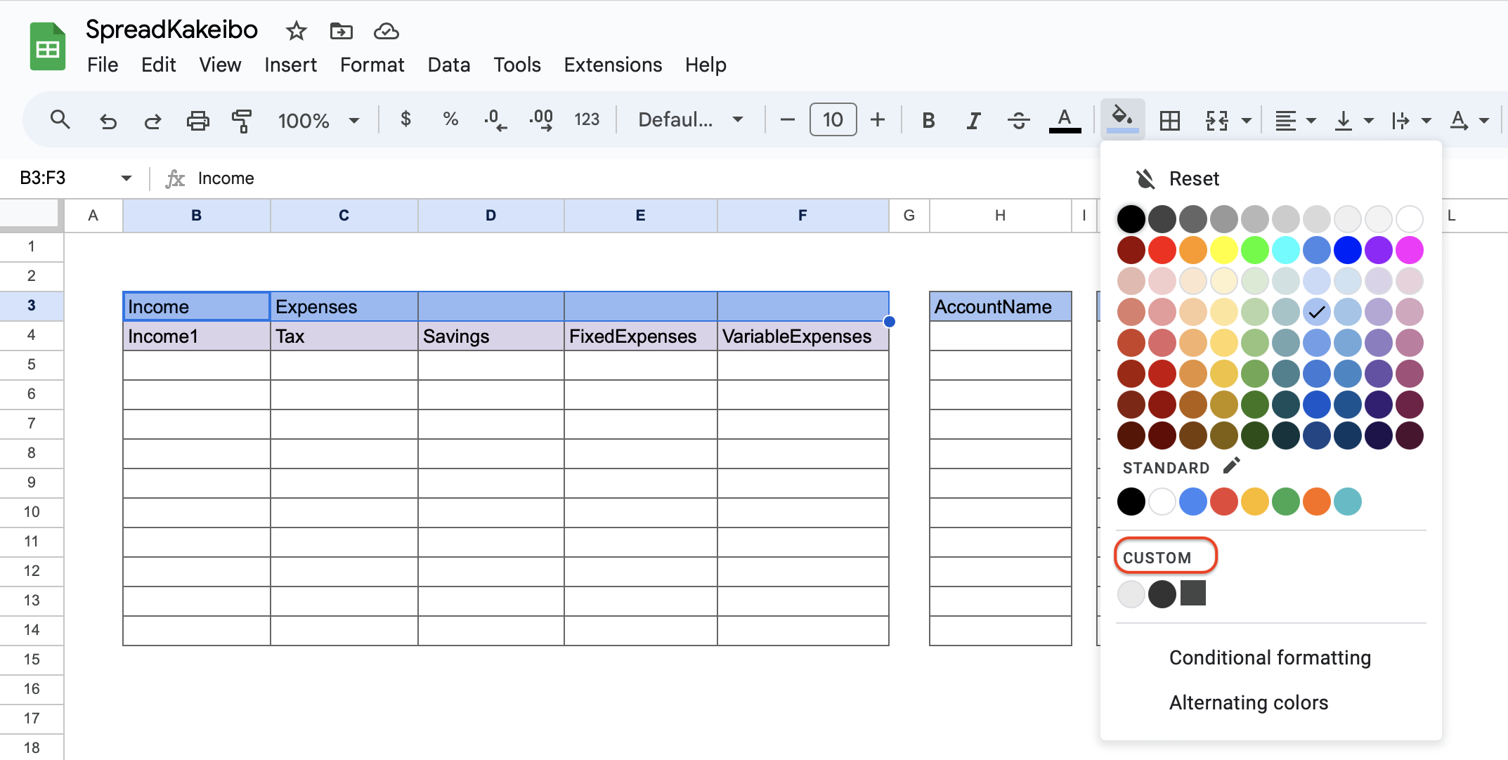
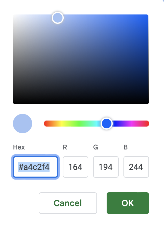
If you do not see a color you like, click on "Custom".
Create your original color.

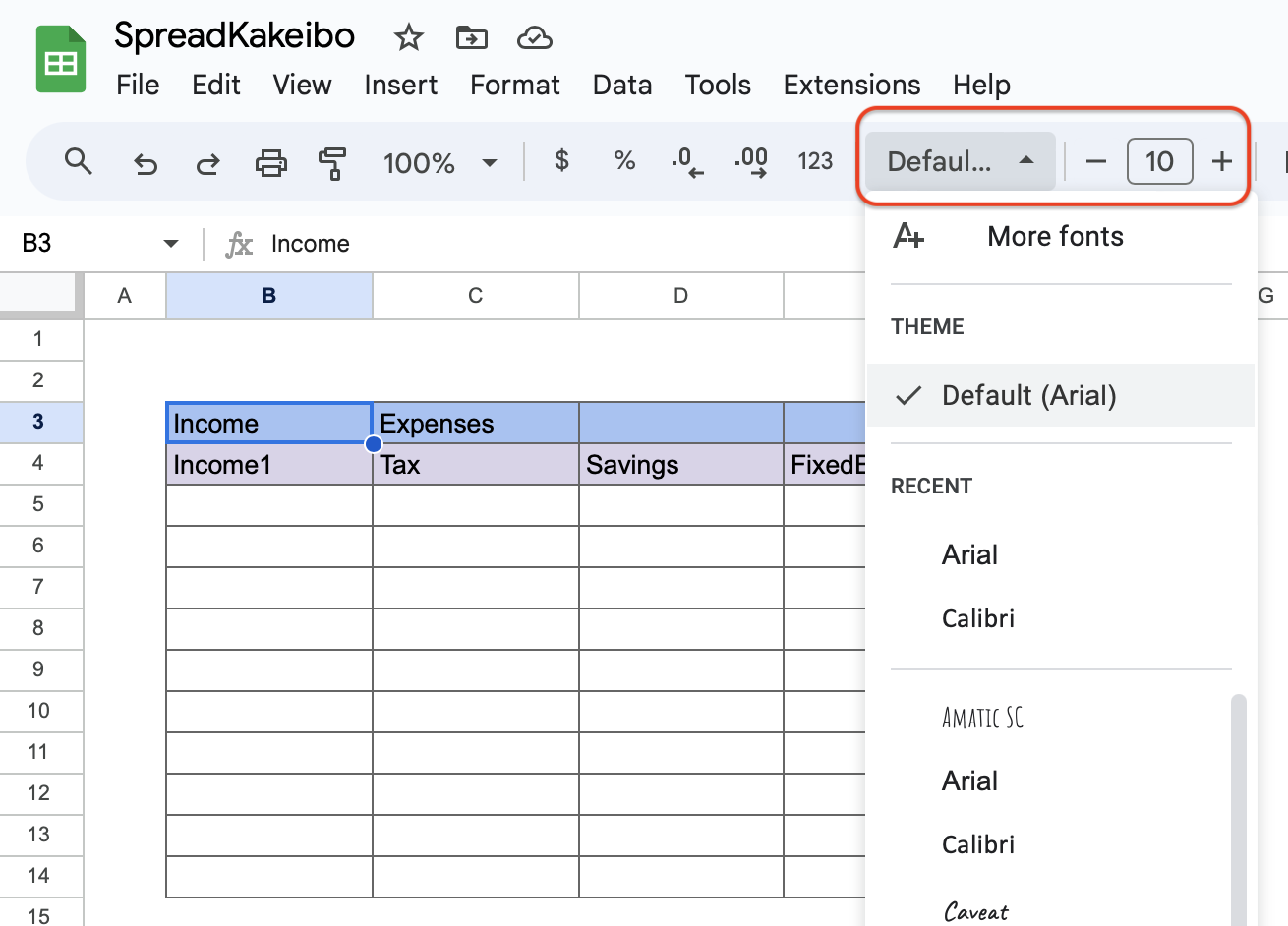
Changing text size and formatting

Click on Text Format and select a format.

Change the font size by clicking the "+" or "-" button or typing the font size directly.

Entering sample values

Sample values are required when creating the input sheet.

After the framework is created, sample values are input.

Input sheet

Add sheets and remove naming and grid lines. (See What to do at the beginning of a setup sheet)

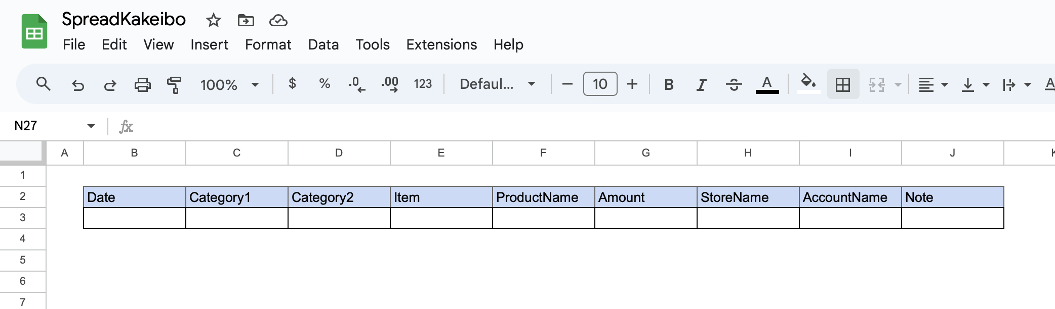
Creating a heading line

• Date: Show calendar
• Category 1: Select income or expenses
• Category 2: Select from Income 1, Taxes, Savings, Fixed Expenses, or Variable Expenses
• Item: Displays the name of each Item 2 expense
• Product name: manually entered
• Amount: Enter manually
• Store name: display the name of the store you set up
• Account: Display the name of the account you set up

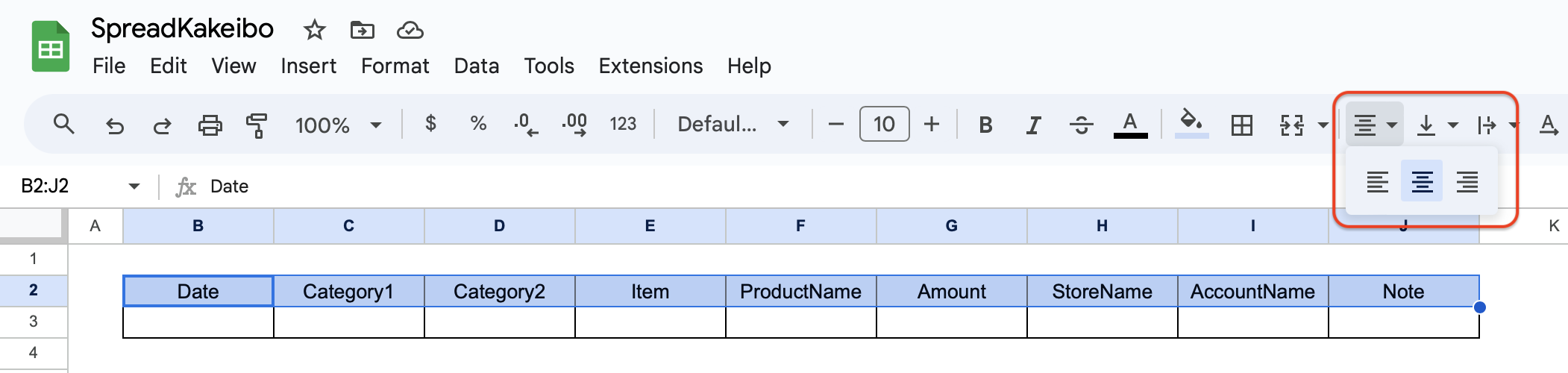
Create a heading line, change the framework and background color.

To change the placement of text, select a range and click on "Horizontal Placement".

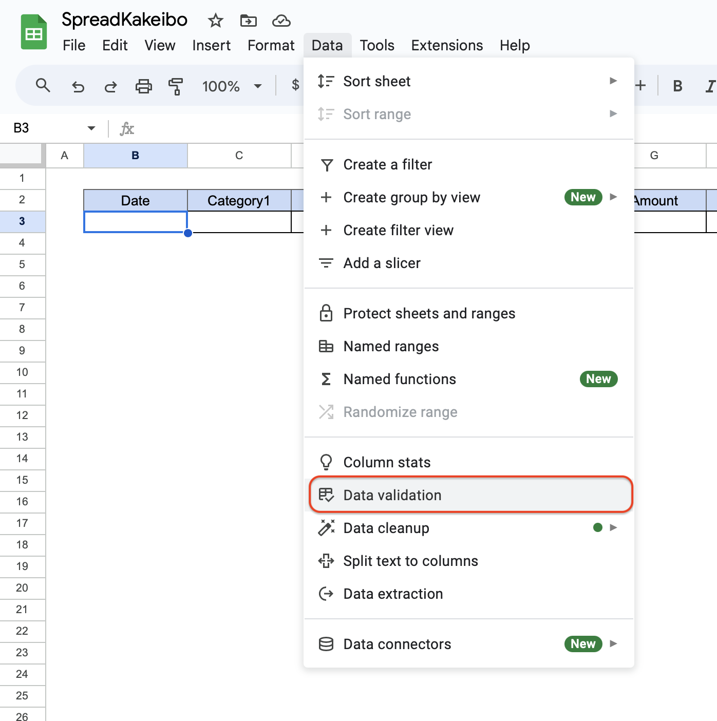
Set date

Display the calendar in the Date column.

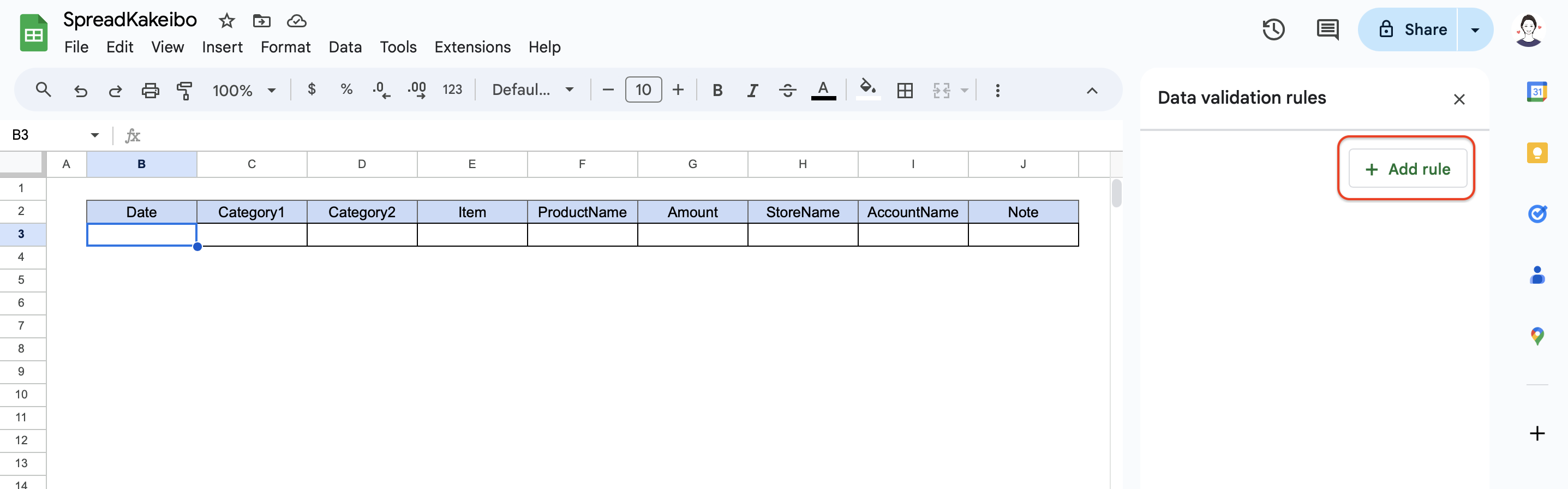
Click on cell B3 and select "Data Validation" under "Data".

Click on "+Add Rule."

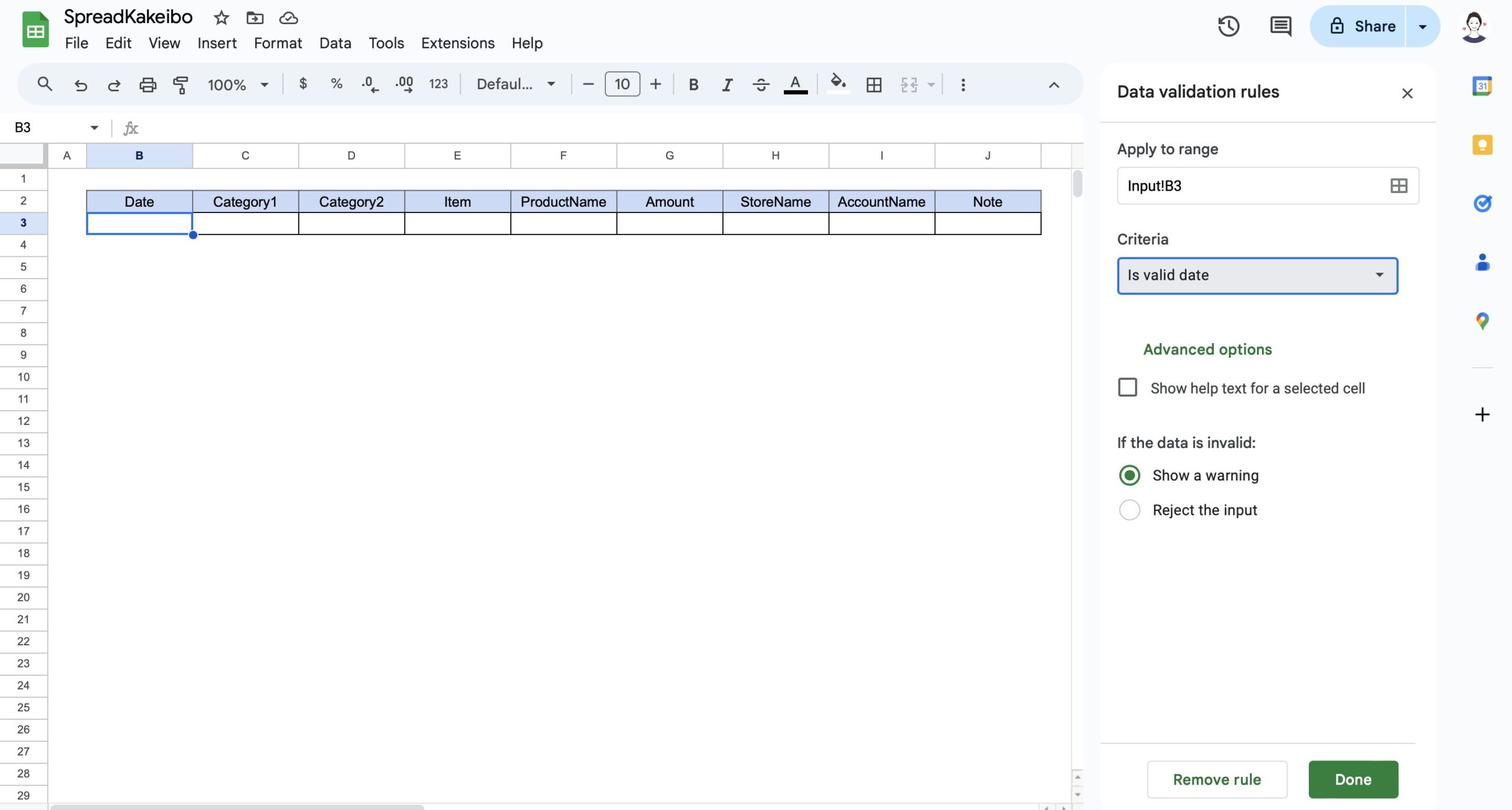
Click on "Is valid Date" from the Criteria section and click the Done button.

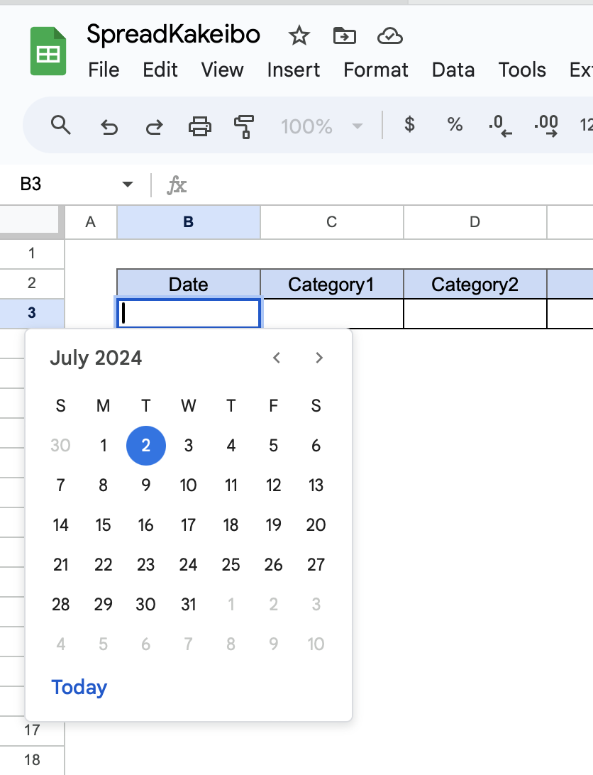
Double-click cell B3 to display the calendar.

Setting Category1

In Category 1, set the tabs so that you can choose between income or expenses.

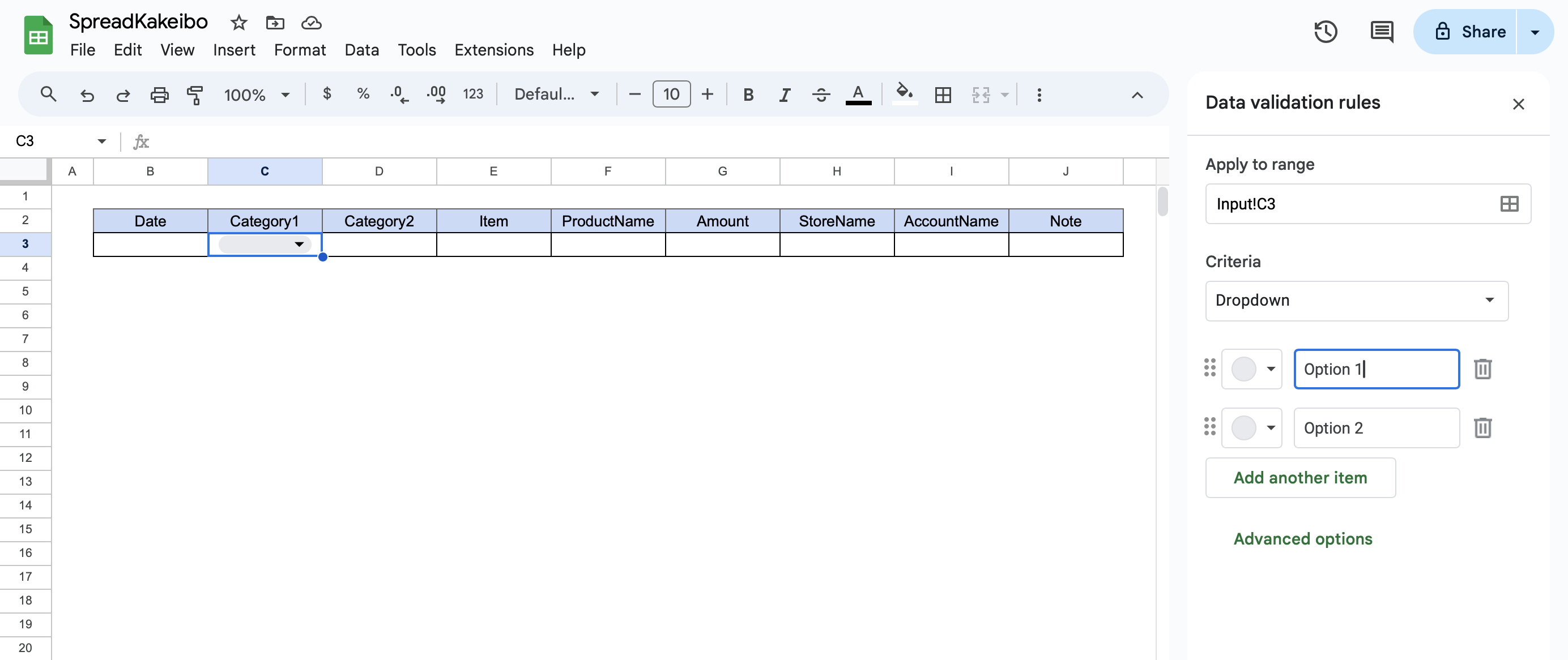
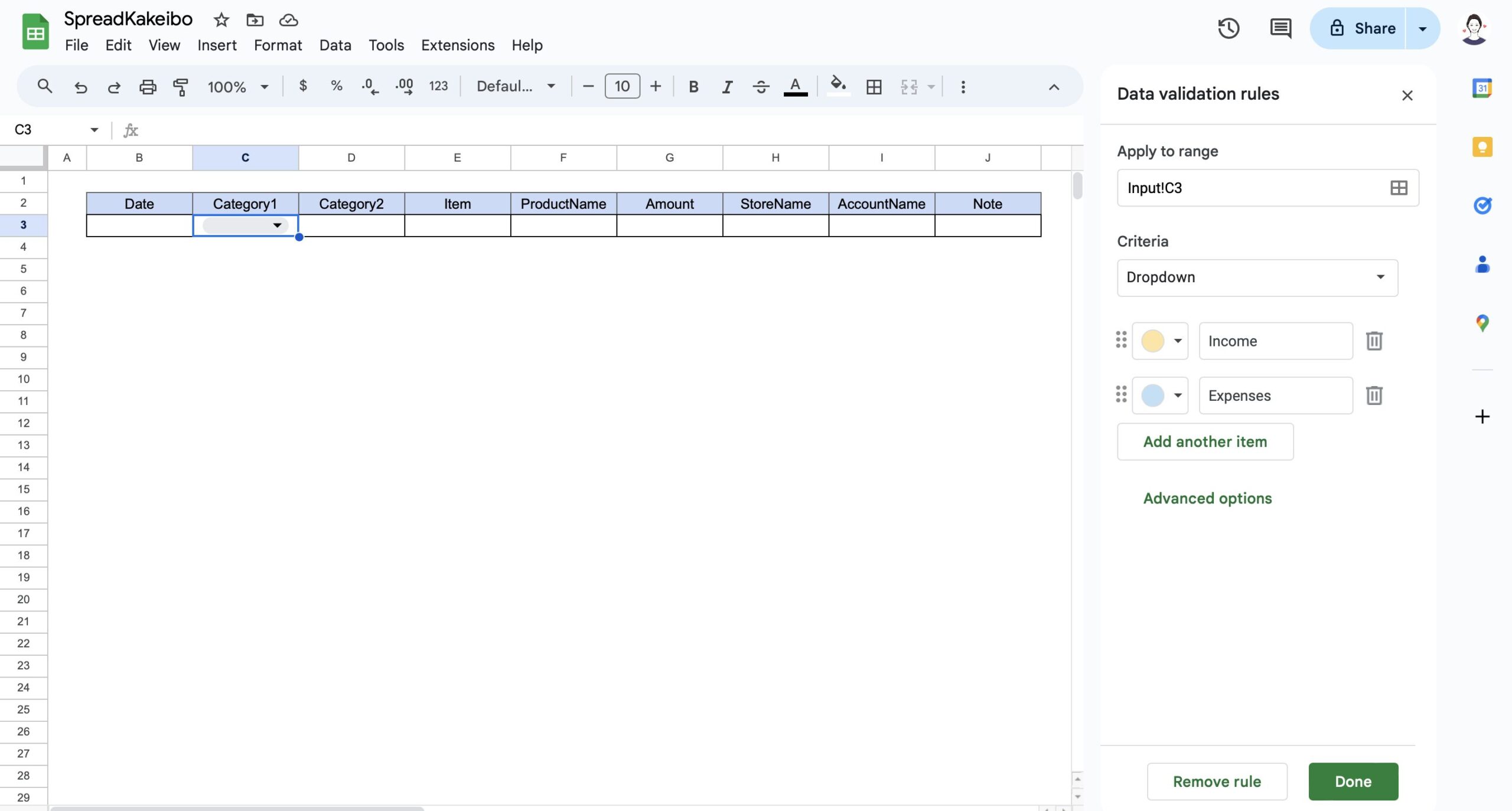
Click on cell C3, click on "Data", then "Data Validation".
Click on "+ Add Rule." (Same procedure as in Calendar Setup)

For the Condition item, make it a "Dropdown" and enter "Income" for Option 1 and "Expense" for Option 2.

If you use the color buttons to the left of income and expenses to change the color, they will be colored when you select from the tabs.

Click the "Done" button.

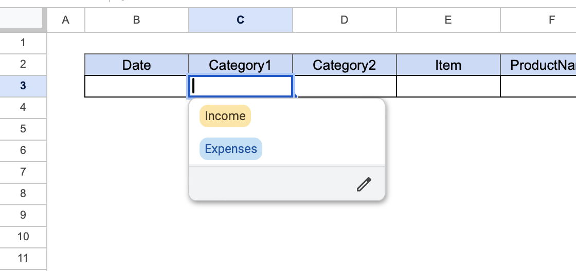
A tab will be added to cell C3, allowing you to select "Income" and "Expenses".

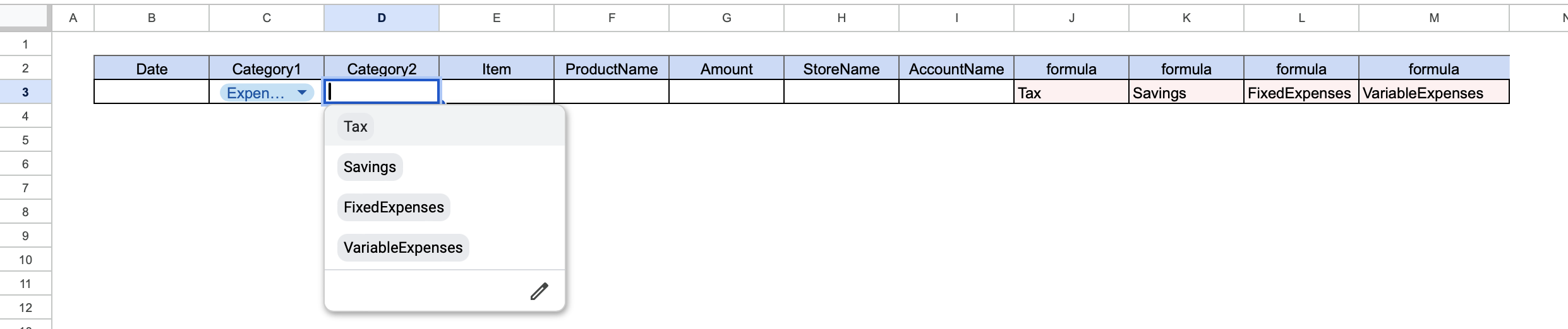
Setting up Category2

Category 2 should allow the user to select from "Income 1" if category 1 is income, and "Taxes, Savings, Fixed Expenses, Variable Expenses" if category 2 is expenses.

In Excel, this can be easily set up using a function, but the spreadsheet does not have this capability.

So, using columns K through N, if category 1 is income, column K will show "Income 1" and if category 1 is expenses, columns K through N will show "Taxes, Savings, Fixed and Variable Expenses".

Then set the values in columns J to M to be selectable from the tabs.

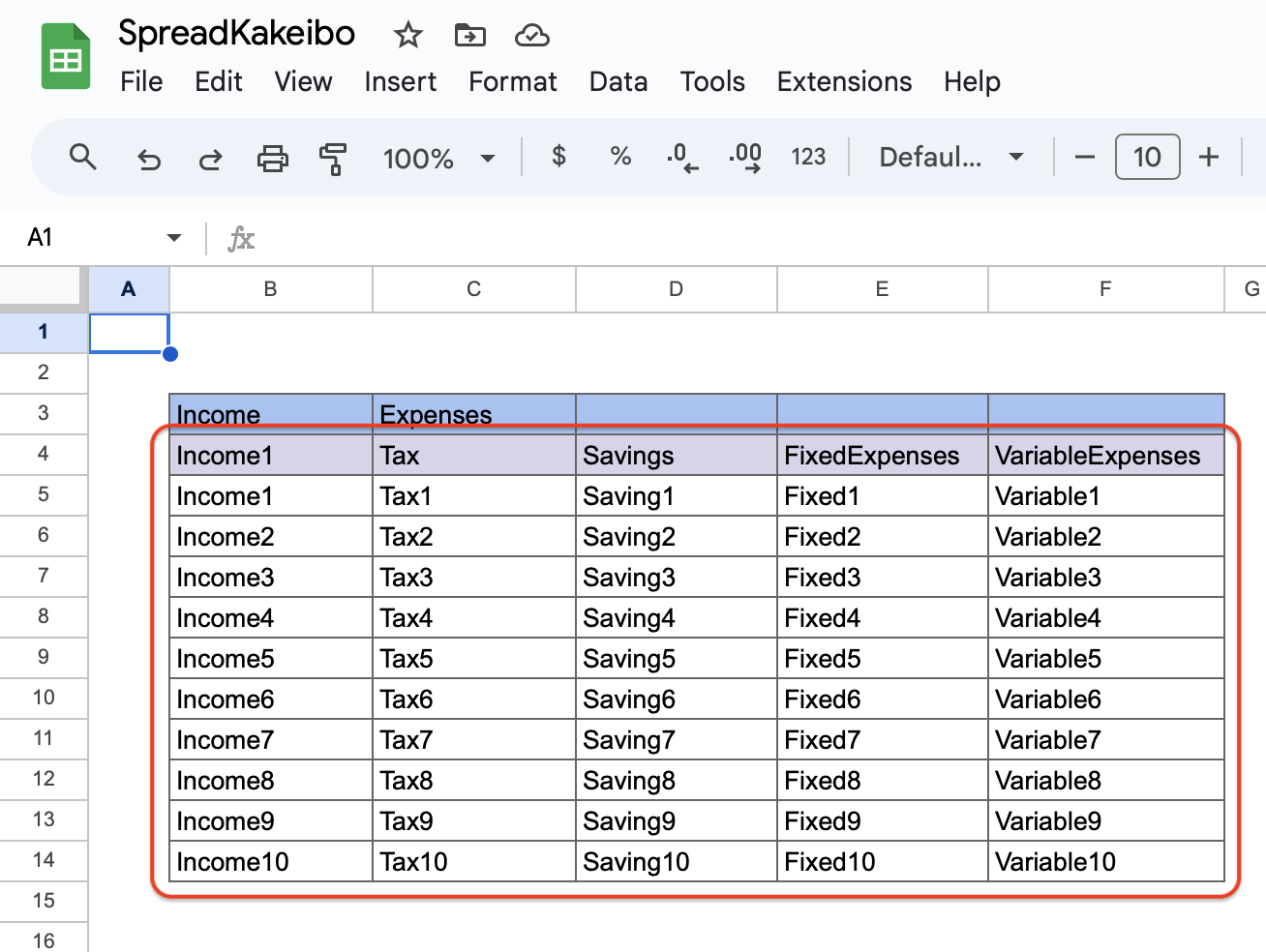
Setting Item Names

Use the available space on the setup sheet to set the item names.

• Income: Income 1
• Expenses: Taxes, Savings, Fixed Expenses, Variable Expenses

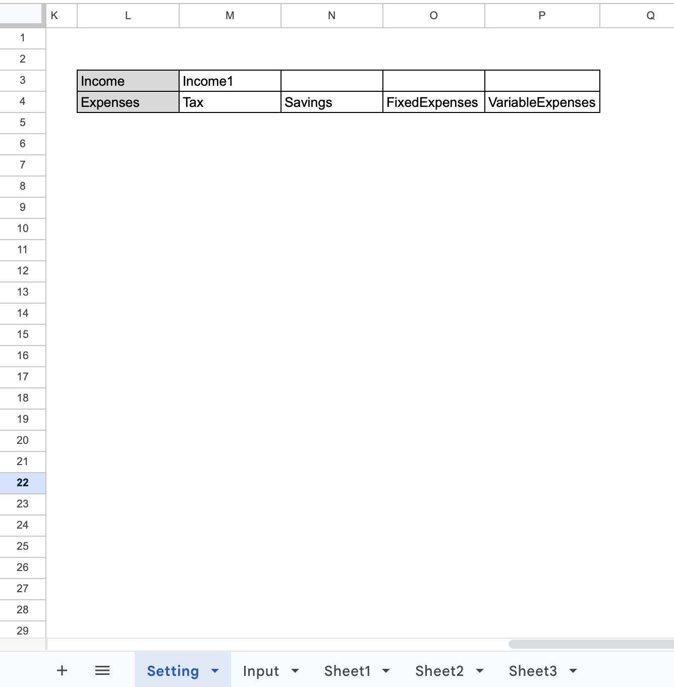
Set up a frame for entering formulas in columns K through N of the input sheet.

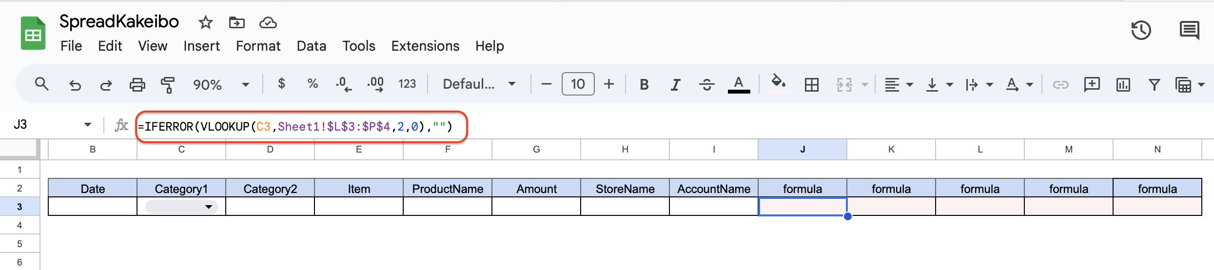
Entering Formulas

Use the VLOOKUP function, which has the ability to search in the vertical columns (income and expenses) and retrieve specific data (income 1 or taxes, savings, fixed expenses, variable expenses).

In column K, enter the formula so that "Income 1" appears if category 1 is income and "Taxes" appears if category 1 is expenses.

=VLOOKUP(C3,'settings'! $L$3:$P$4,2,0)

The range is dragged from L3 to P4 on the settings sheet.
Fix with $ mark to prevent shifting when copying and pasting ($L$3:$P$4)

For the search, enter "0" to display only exact matches.

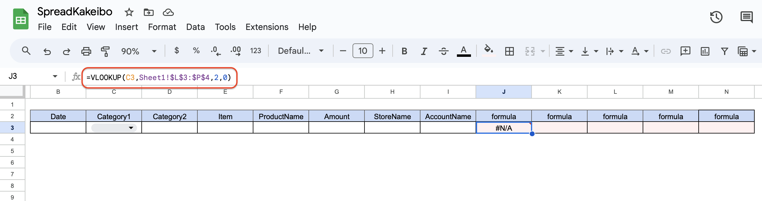
If category 1 is blank, an error is displayed.

If you are concerned about the error message, use the IFERROR function to blank it out.

=IFERROR(VLOOKUP(C3,'setting'! $L$3:$P$4,2,0),"")

Function to blank on error.

The "" is the symbol for whitespace.

Copy and paste J3 into column K to M.

C3 will be displaced, so correct to C3.

Add the column numbers by 1. (K is 3, L is 4, M is 5)

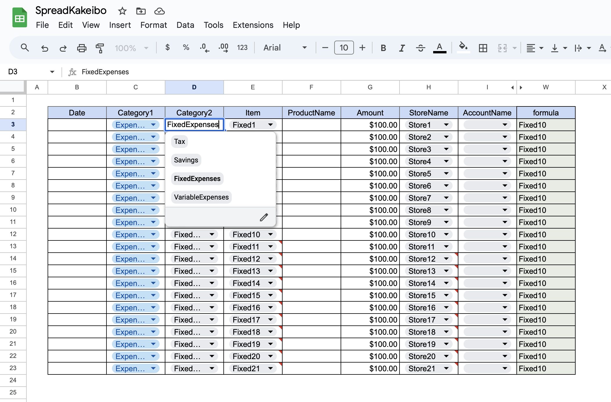
Set tabs on category 2

Click on cell D3 and select "Data" and "Data Validation".

For the Criteria, select "Dropdown (from a range)".

Select J3 to M3 from the data range selection below it and click the "Done" button.

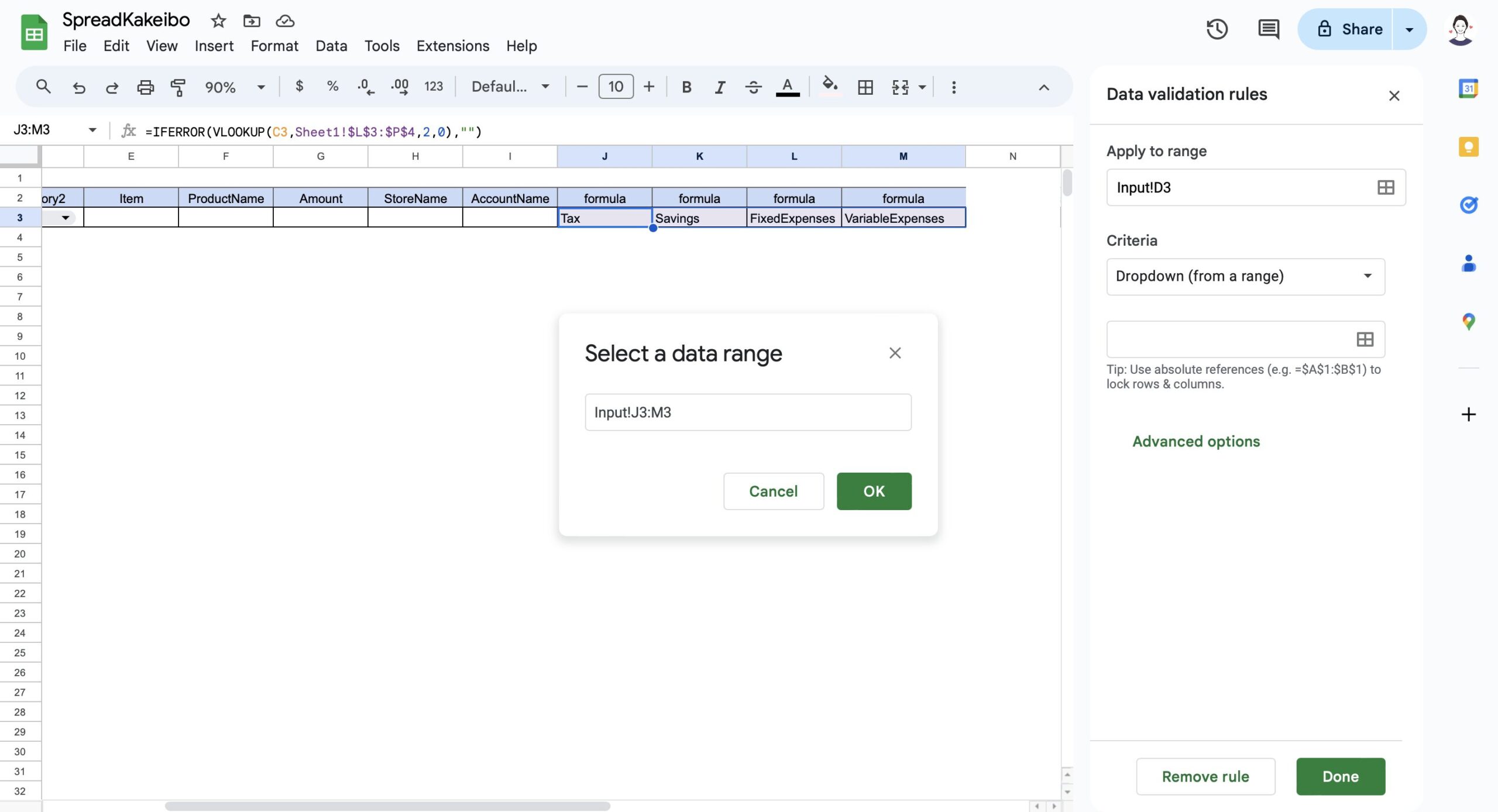
A tab is added to cell D3 and the item name is displayed according to the contents of category 1.

Setting up Item

Create a formula column similar to the one set up for Category 2 to display the expense item names according to Category 2.

The range used in the formula is from B4 to F14on the setup sheet.

Creating Formula Columns

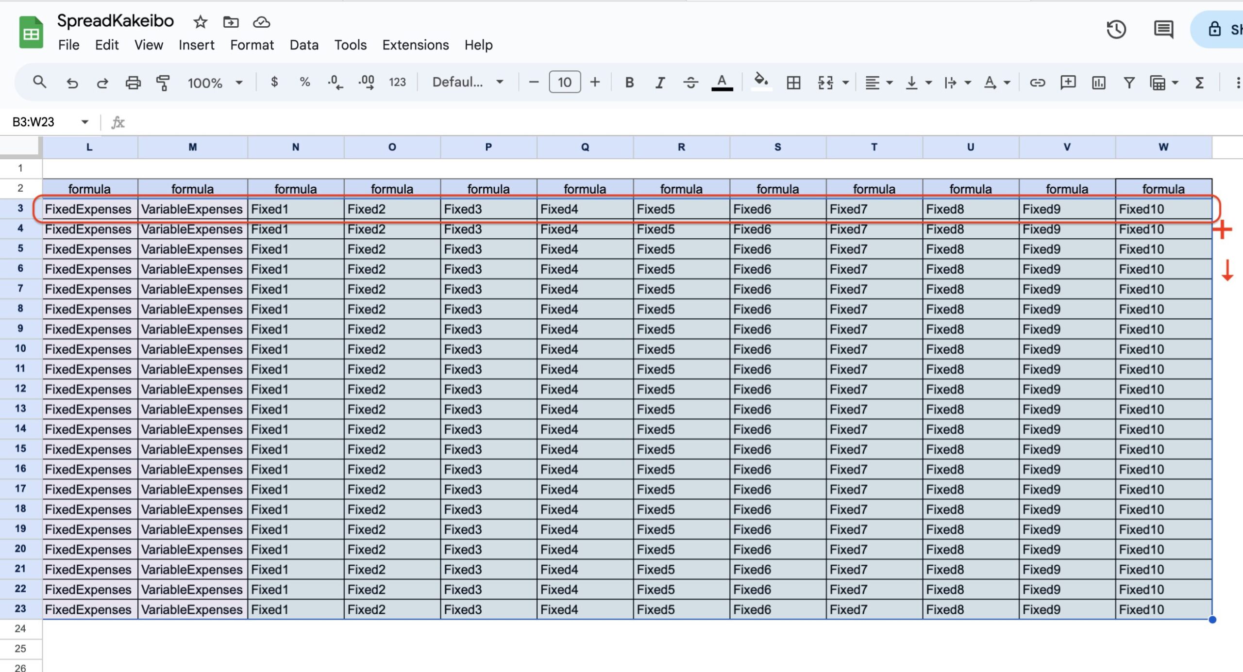
Since up to 10 expense item names can be registered, create 10 columns of formula frames (from column N to W).

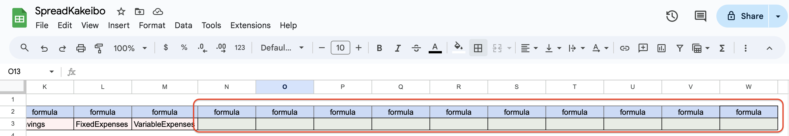
Entering Formulas

Use the HLOOKUP function, which has the ability to search in the horizontal columns (Income 1, Taxes, Savings, Fixed Expense, Variable Expense) to retrieve specific data (expense item names).

In column N, enter the formula so that Income1, Taxe1, Saving1, Fixed1, and Variable1 are displayed according to the contents of category 2.

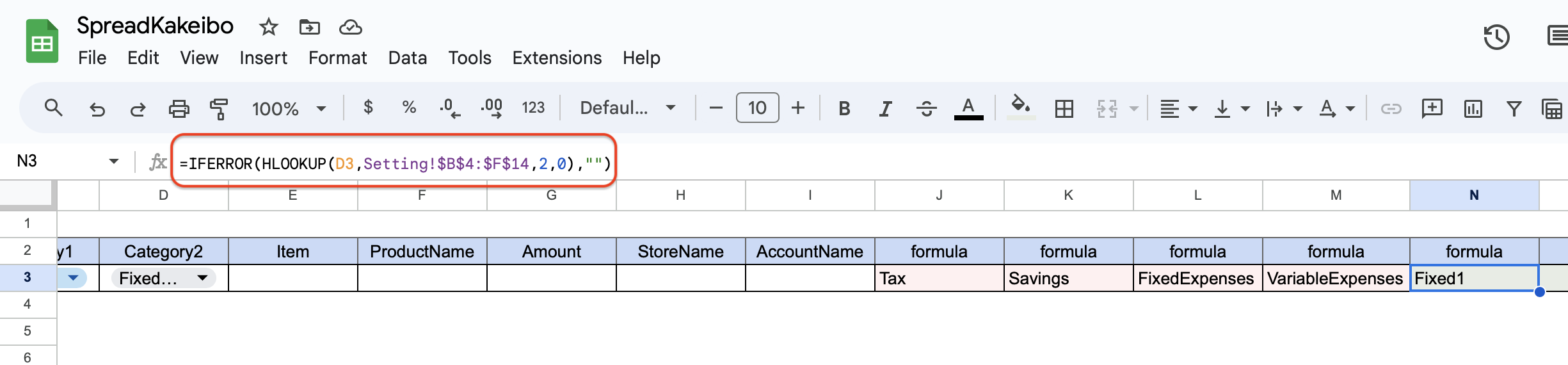
=IFERROR(HLOOKUP(D3,'setting'! $B$3:$F$13,2,0),"")

Similar to setting category2, enter IFERROR("") to avoid errors.

Drag the range from B4 to F14 on the settings sheet.
Fix with a $ mark to prevent shifting when copying and pasting ($B$4:$F$14)

For the search, enter "0" to show only exact matches.

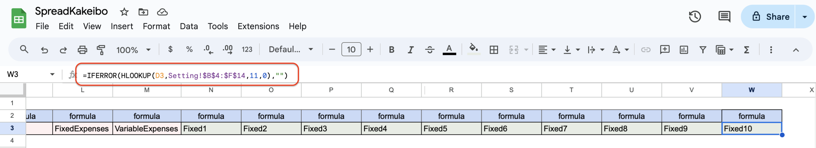
Paste the formula for N3 from column O to column W.

The search value D3 will be out of place, so correct it to D3.

Add the row numbers one by one from the left.

The row number for W3 will be 11.

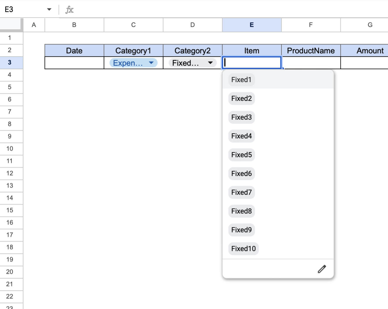
Set tabs for expenses.

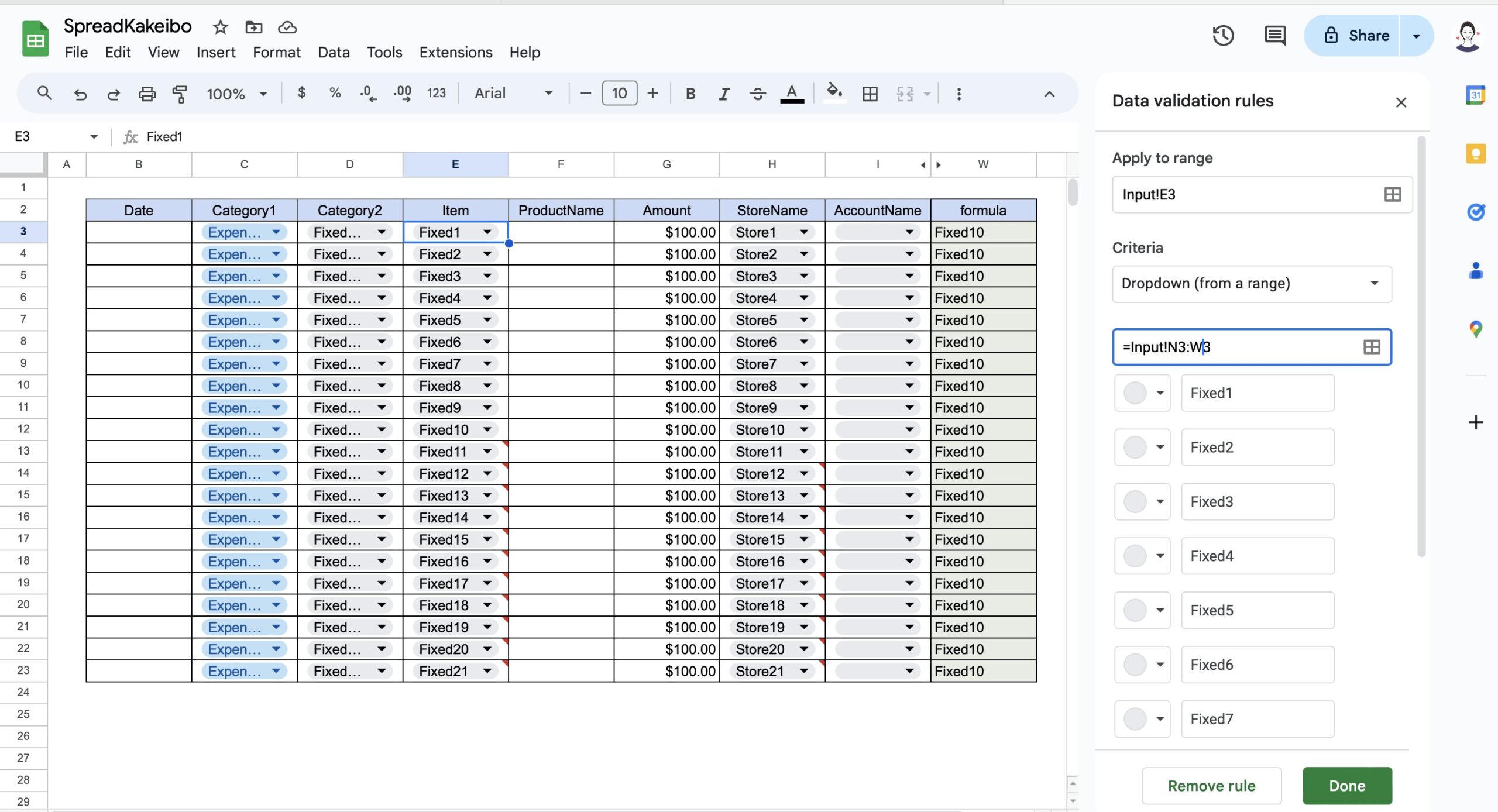
Click on cell E3 and select "Data" and "Data validation".

For the Criteria, select "Dropdown (from a range)".

Select N3 to W3 from the data range selection below it and click the "Done" button.

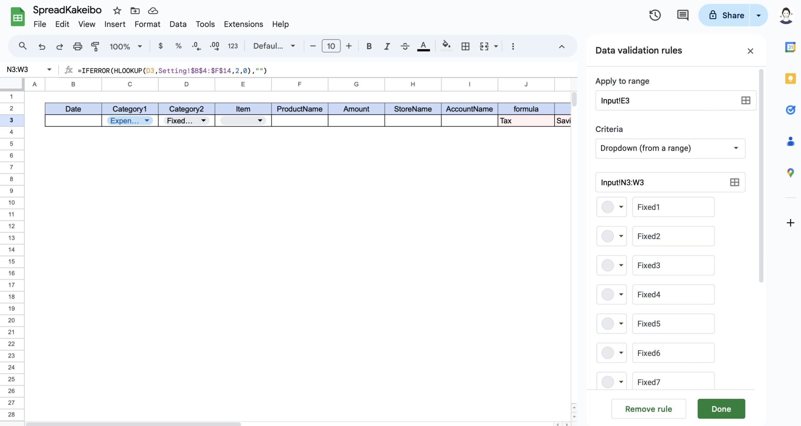
A tab will be added to column E and the expense item name in item 2 will be displayed.

Adding currency units to the Amount column

Select column G, then select "Display Format," "Number," and "Custom currency.

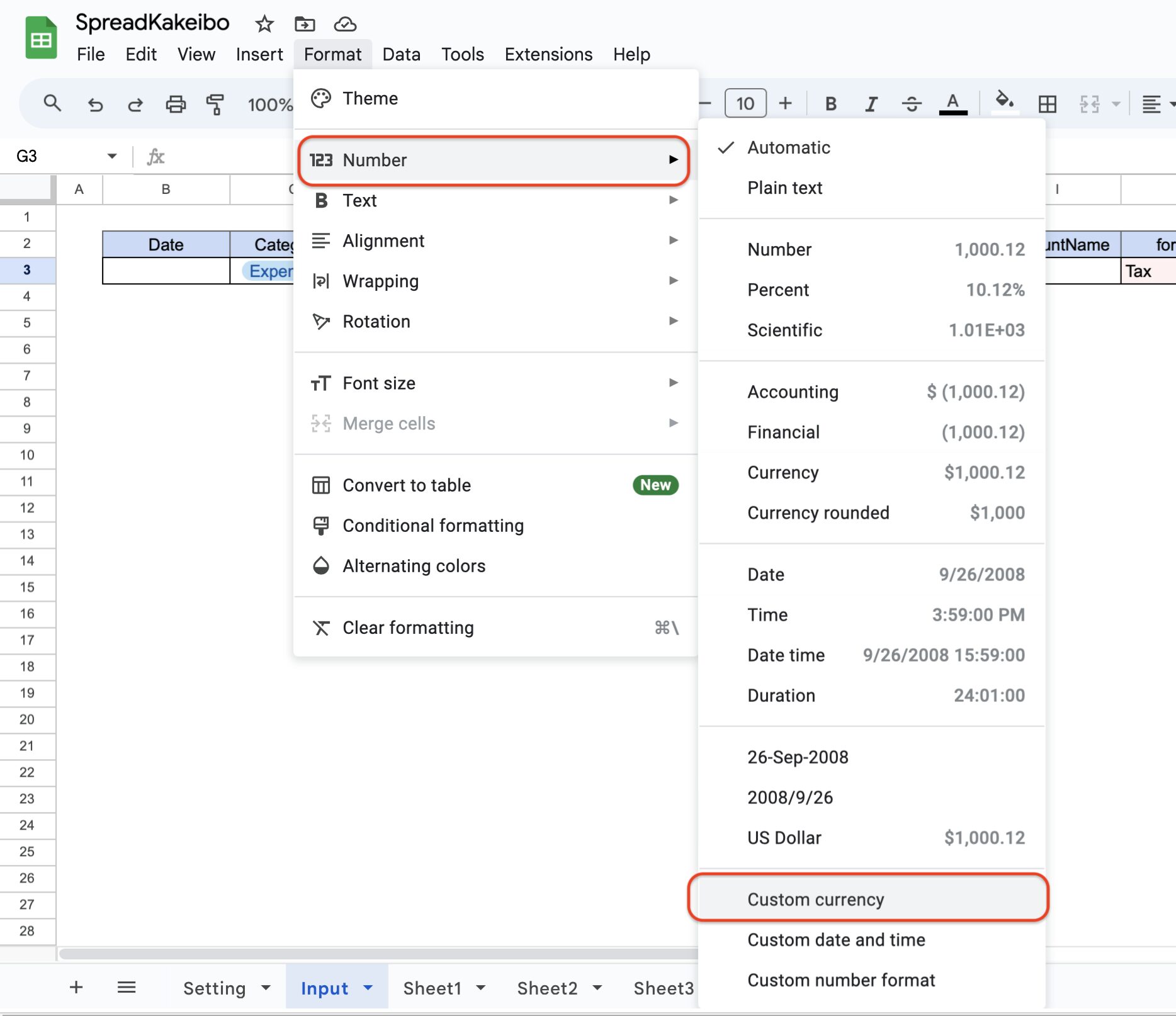
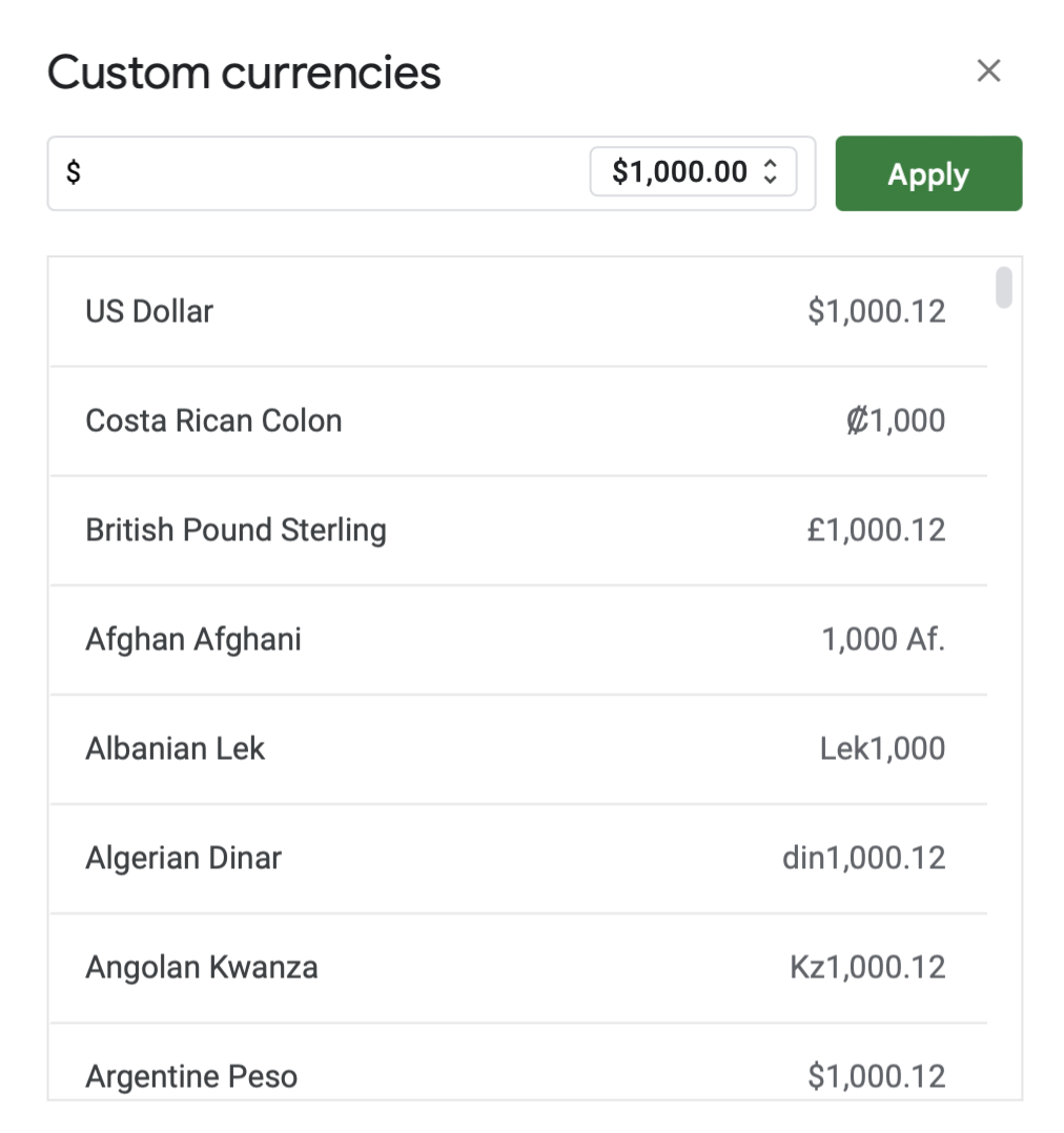
Please select your local currency unit.

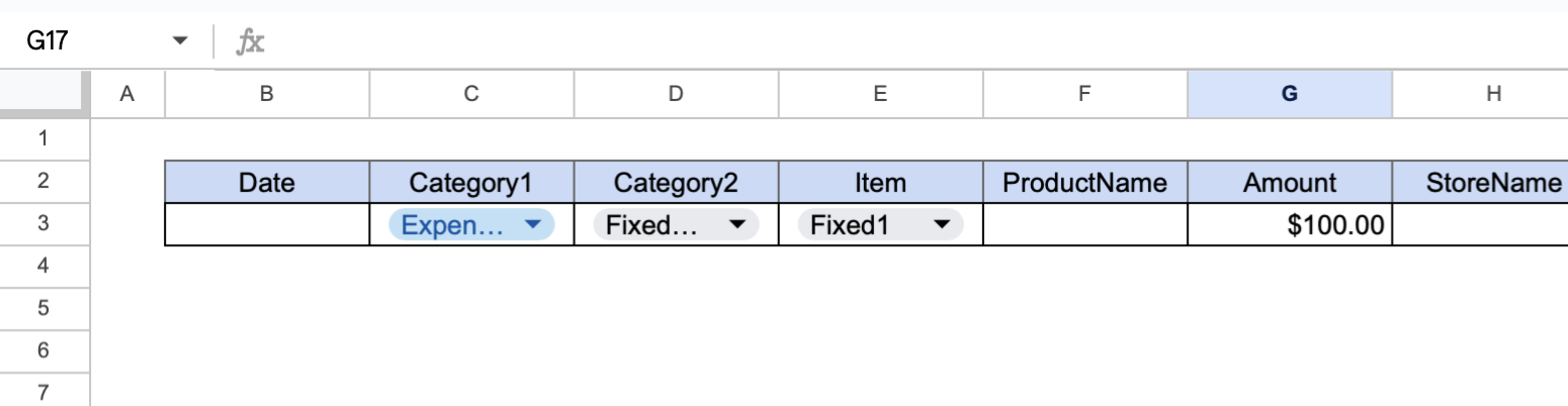
When you enter a number in the amount field, the currency unit is automatically displayed.

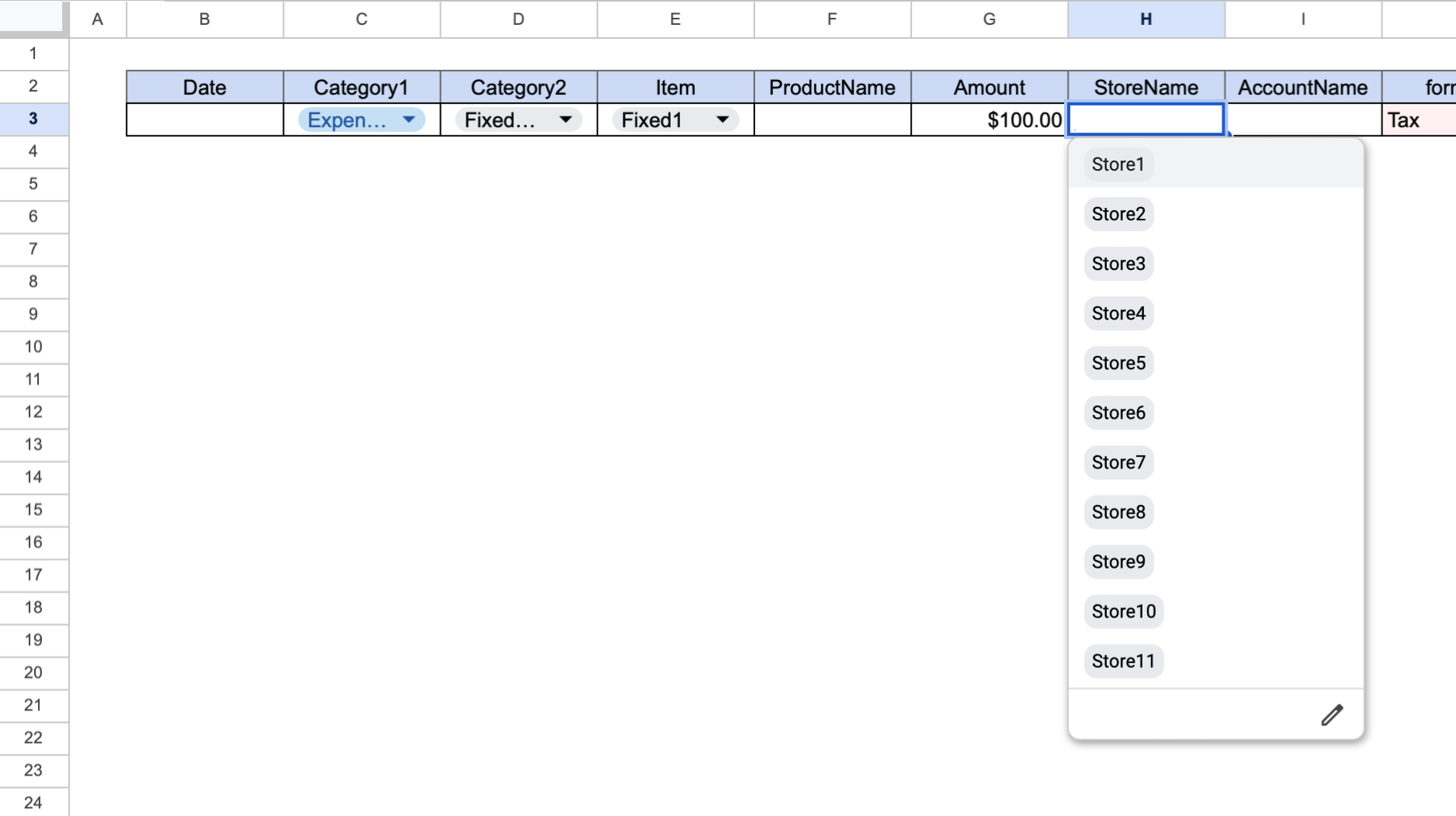
Set up store name and account tabs

Set up a tab for the store name.

Click on H3 and select "Data validation" and "+ Add Rule".

Select the Dropdown(from a range) for the Criteria, and for the range, go to the settings sheet and drag J4 to J14 and click the Done button.

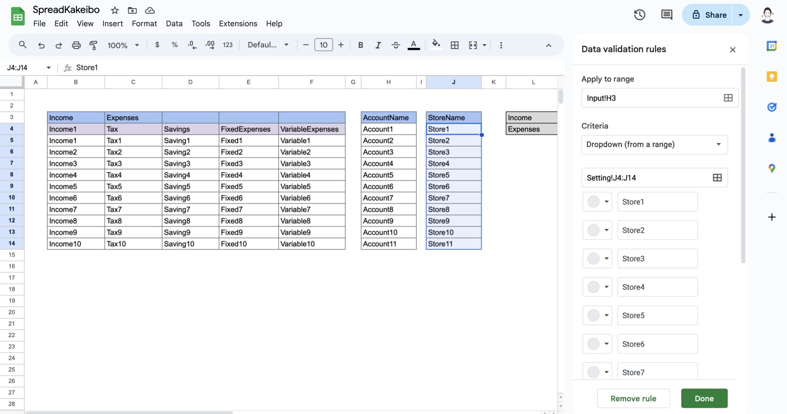
A tab will be added and the name of the store entered in the settings will appear.

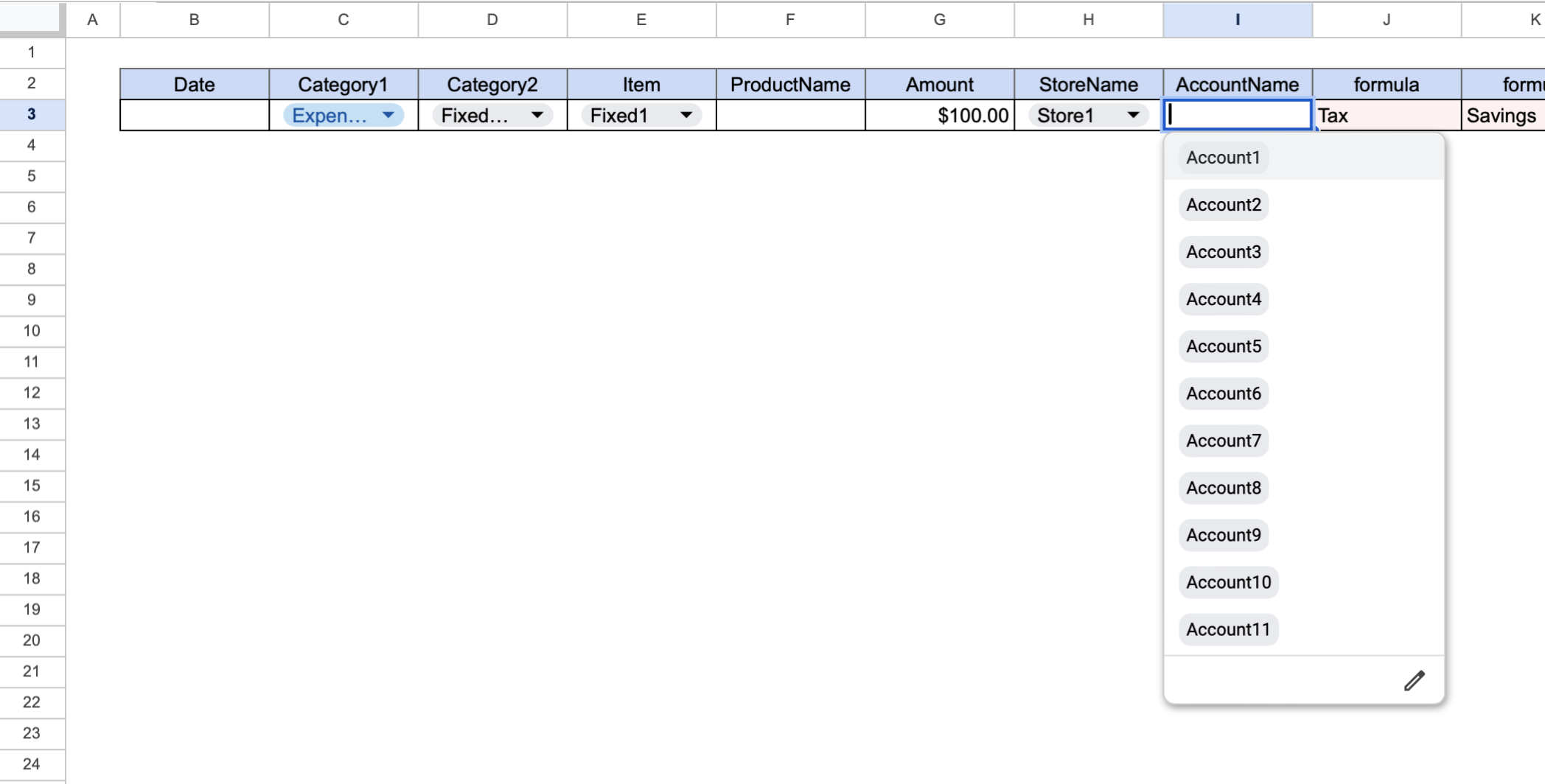
Set tabs for accounts

Click on I3 and select "Data validation" and "+Add rule".

Select the Dropdown(from a range) for the Criteria, and for the range, go to the settings sheet and drag H4 to H14 and click the Done button.

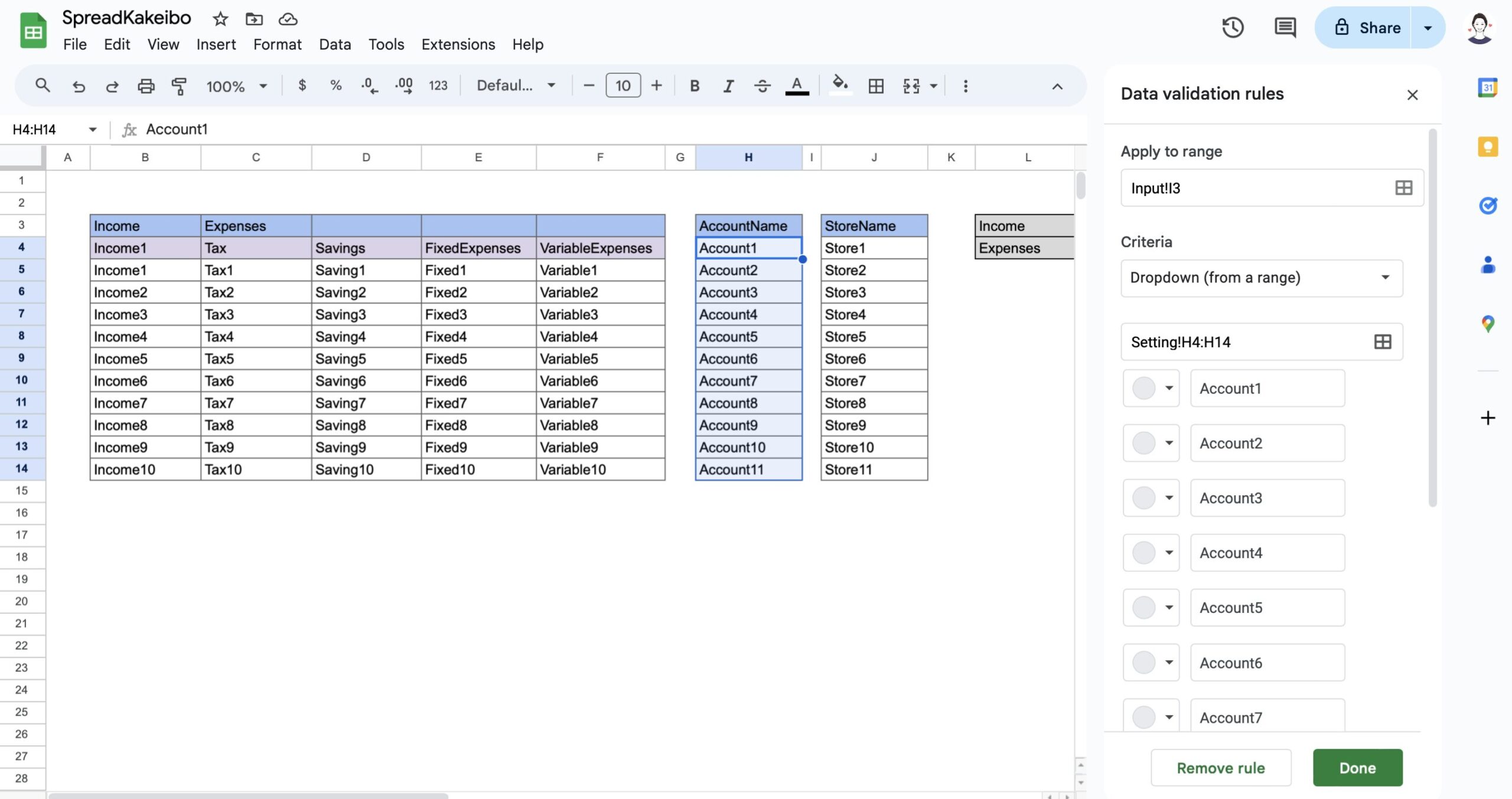
A tab will be added and the account name entered in the settings will be displayed.

Create tables

Copy and paste row 3.

Select cells B3 to W3 and drag and paste below.

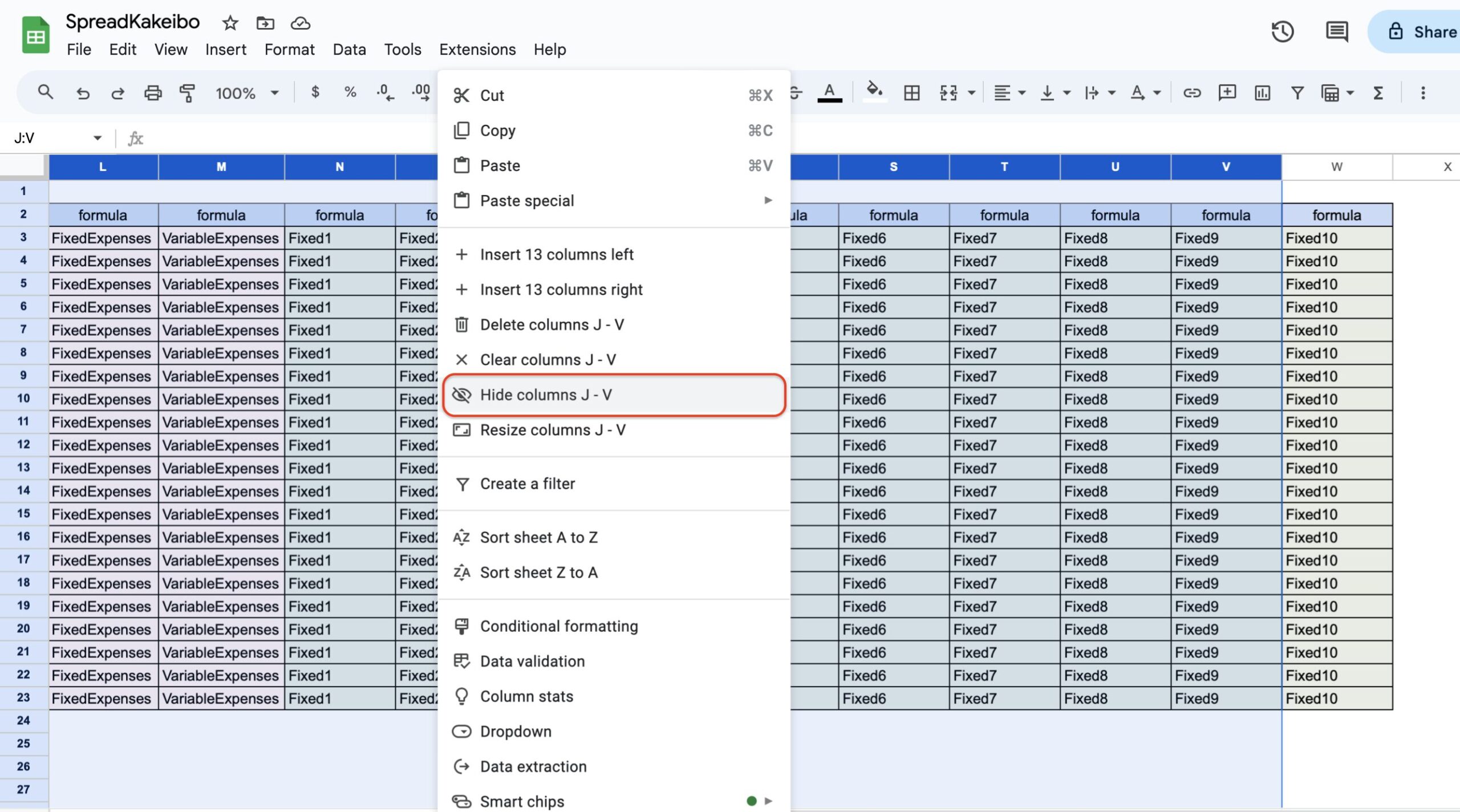
Hide the columns, as these formulas are not needed for daily input.Select columns K to W, right click, and click "Hide Columns J-V".

Leave column W as it will be needed when adding more rows.

Check category 2 and item tabs.

The range of tabs may be fixed, so check them through the edit marks.

Click on the tab for D3 and click on Edit (pen symbol) at the bottom.

The range of data has been fixed with a "$".

If the range is fixed, the range J3 to M3 will be applied to all the rows below.

Erase the dollar signs so that the range for each row is the same.

=Input!J3:M3

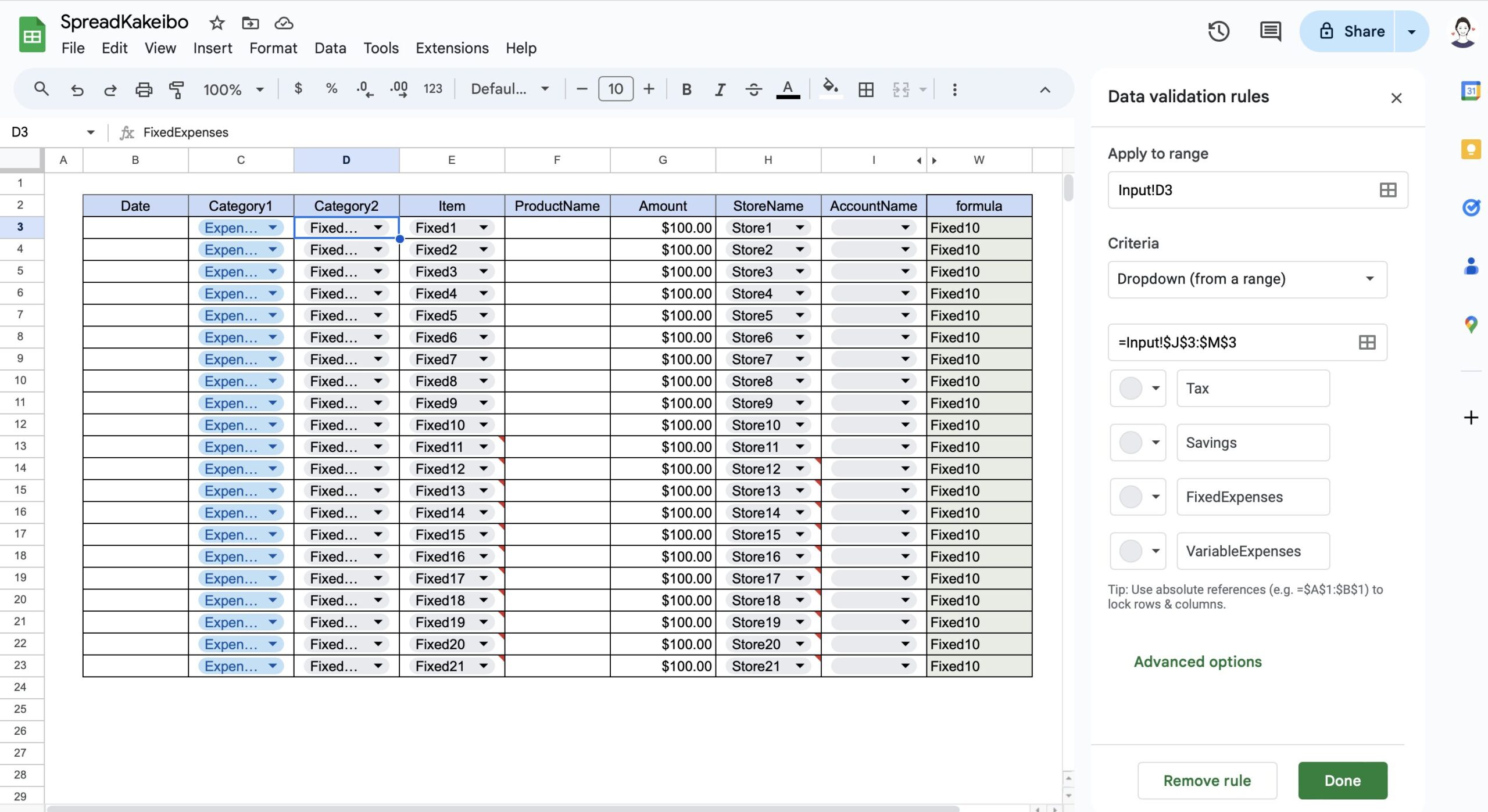
Erase the dollar signs and click Done.

Click "Apply to All" to fix the range for all rows in column D.

The same range is changed for item E3.

Create filters

Set filters to display by expense, store name, account, etc.

Select a heading (B2 to W2).
Click on "Data" and "Create a Filter.

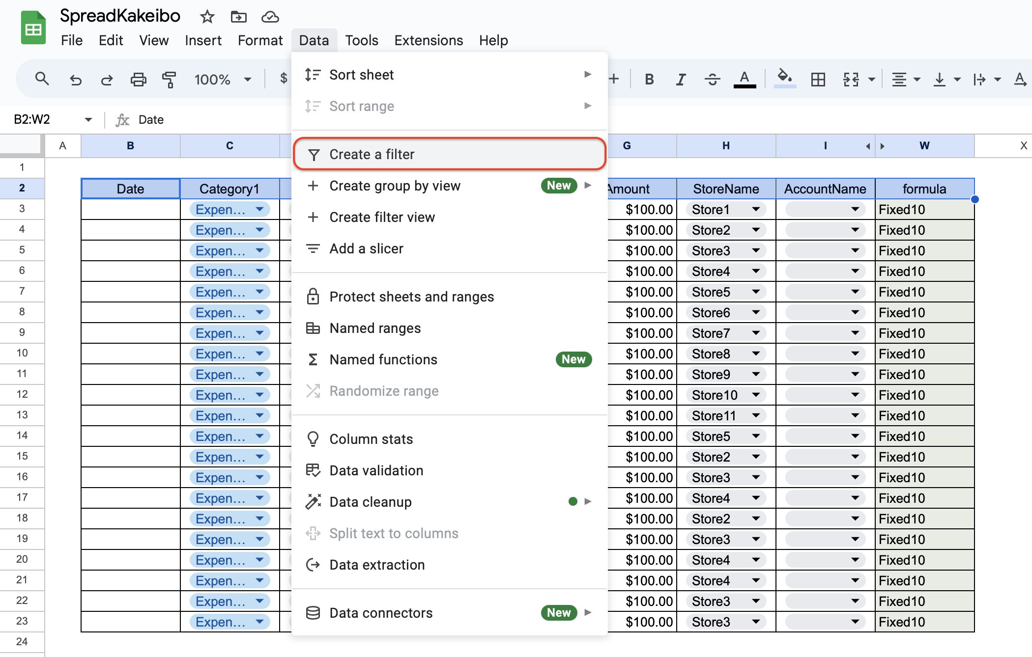
A filter will be added to the heading row.

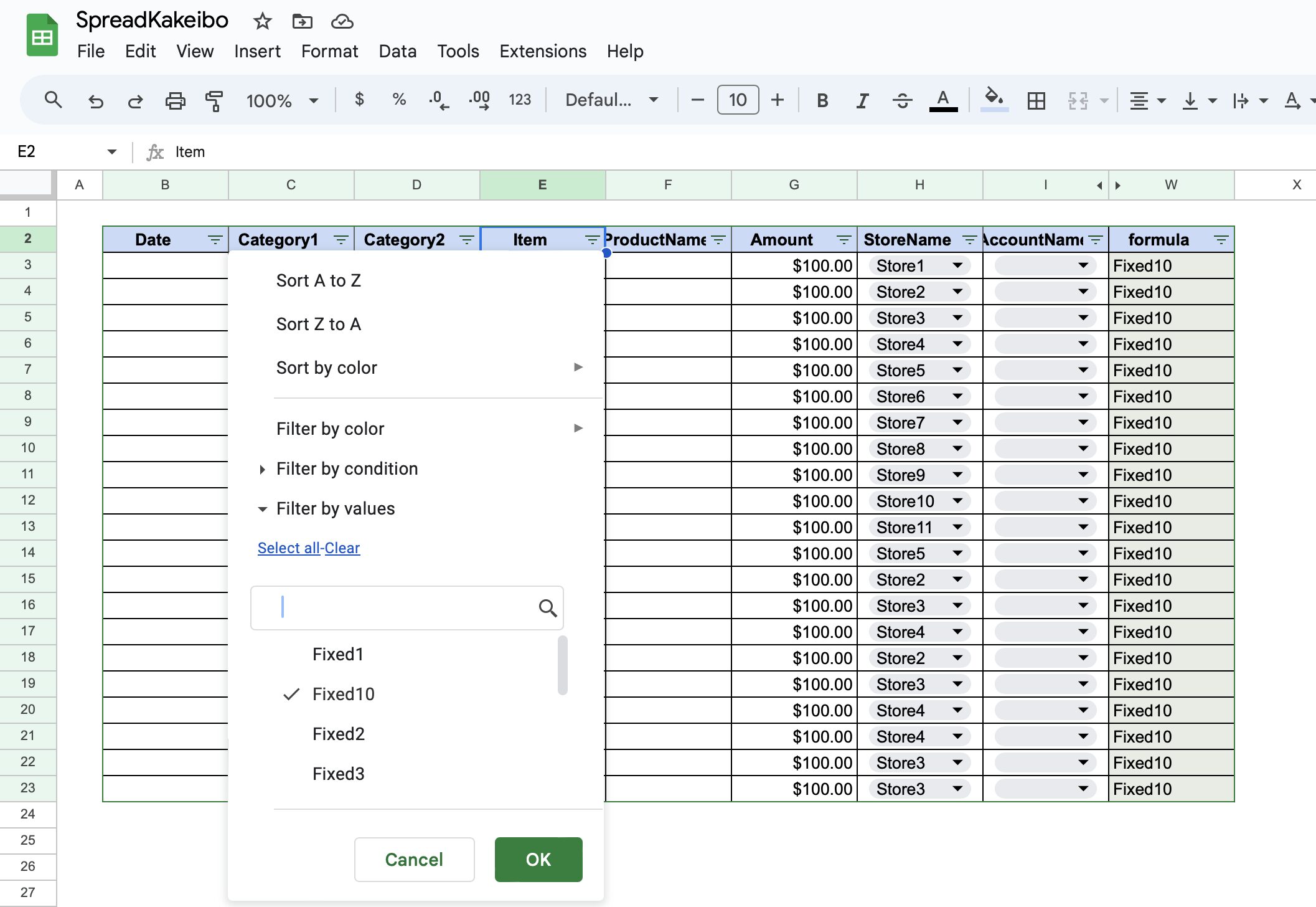
Click on the filter you want to display, click "Clear" and check the items you want to display.

Fix heading rows

Fixing the second row and moving only the rows after it makes daily input easier.

Click on "View," "Fix," and "2 Rows.

Two rows" means that the top two rows are fixed.

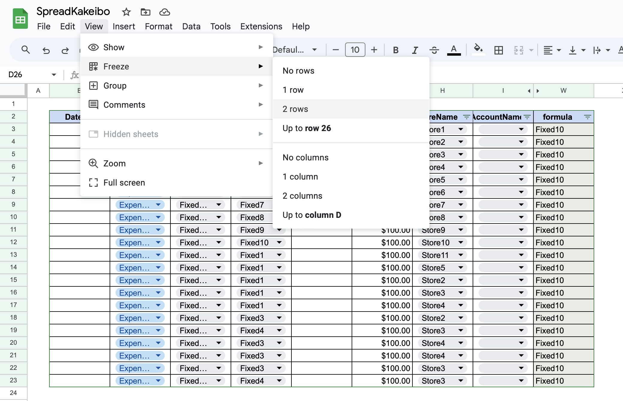
If you scroll down, the heading line will be fixed and only the subsequent lines will move.

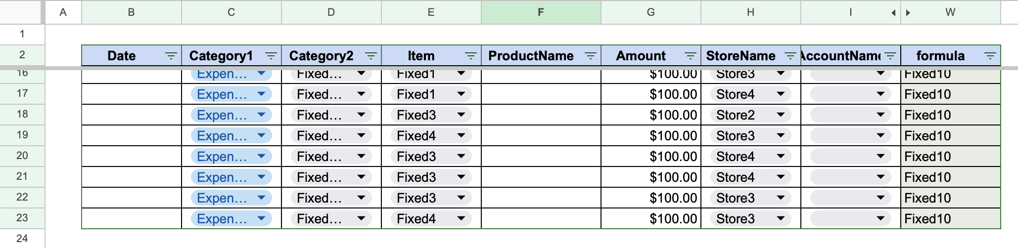
Fixed expense sheet

To make the entry as easy as possible, a fixed cost sheet is provided.

By entering all items other than variable expenses in this column, you can copy and paste this information into the table on the left each month.

Copy input sheet

Right click on the sheet name "Input" and click on "Duplicate".

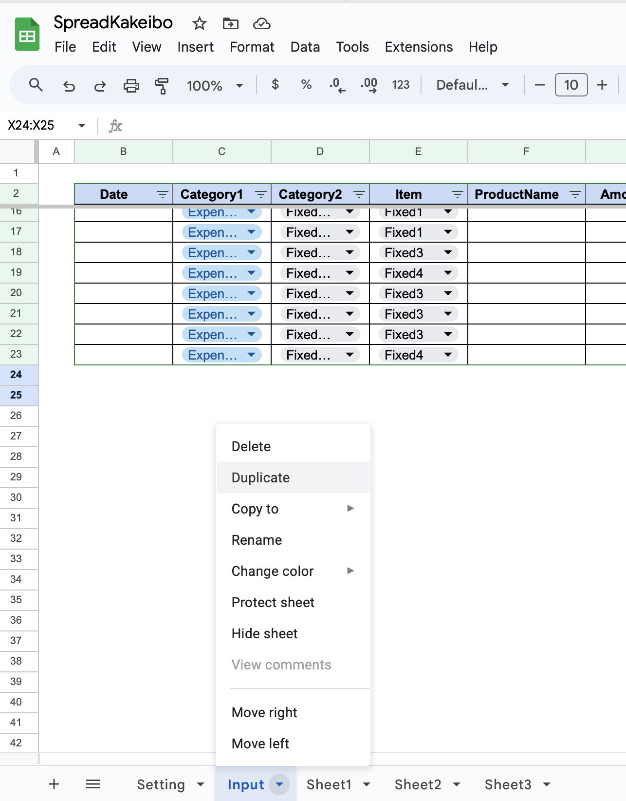
Name the copied sheet.

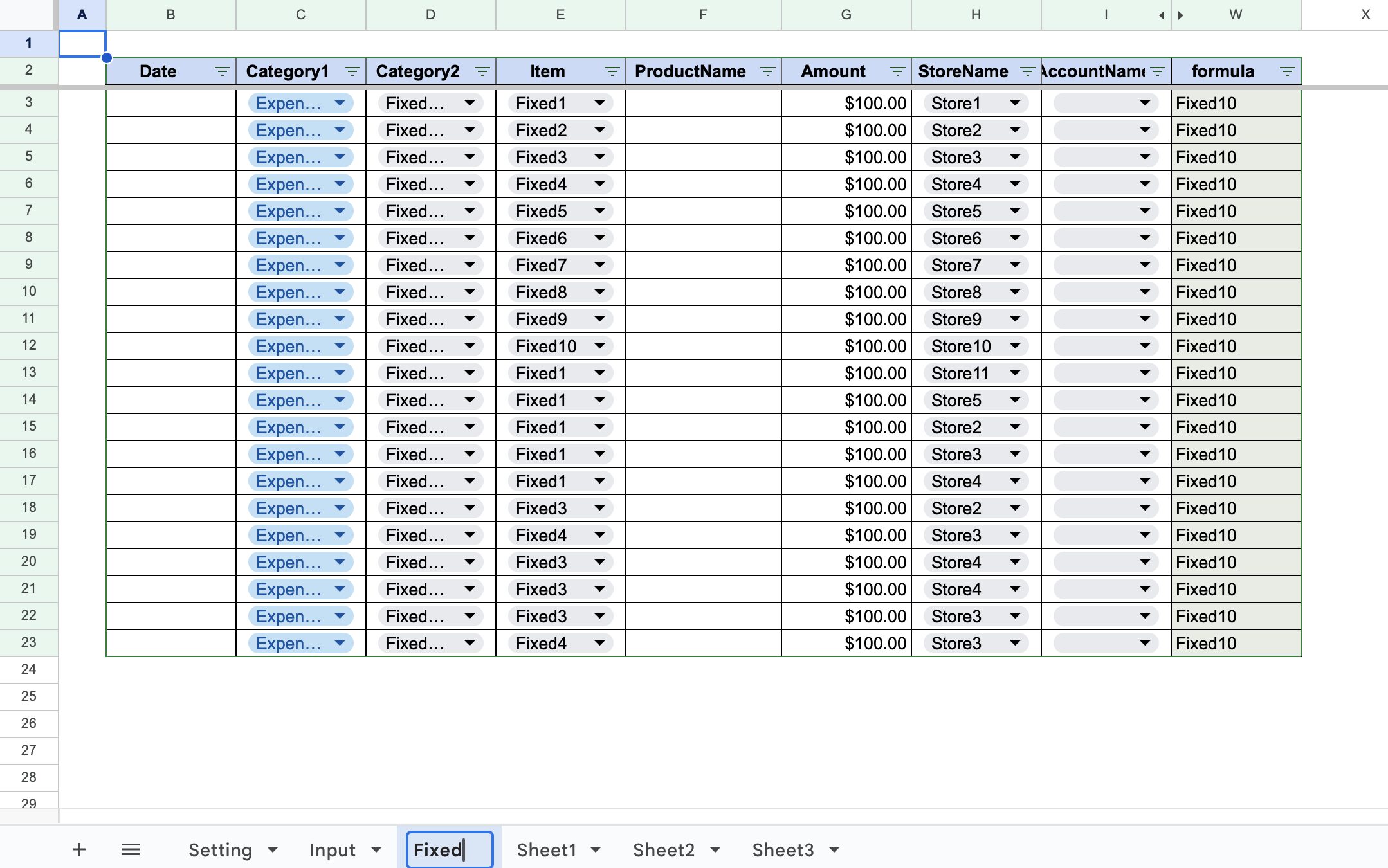
Input sample values

On the Fixed Expenses sheet, enter the items that will be required each month.

Enter sample values as they are needed to create the Income and Expenses sheet.

Leave the date blank and the expense amount negative.

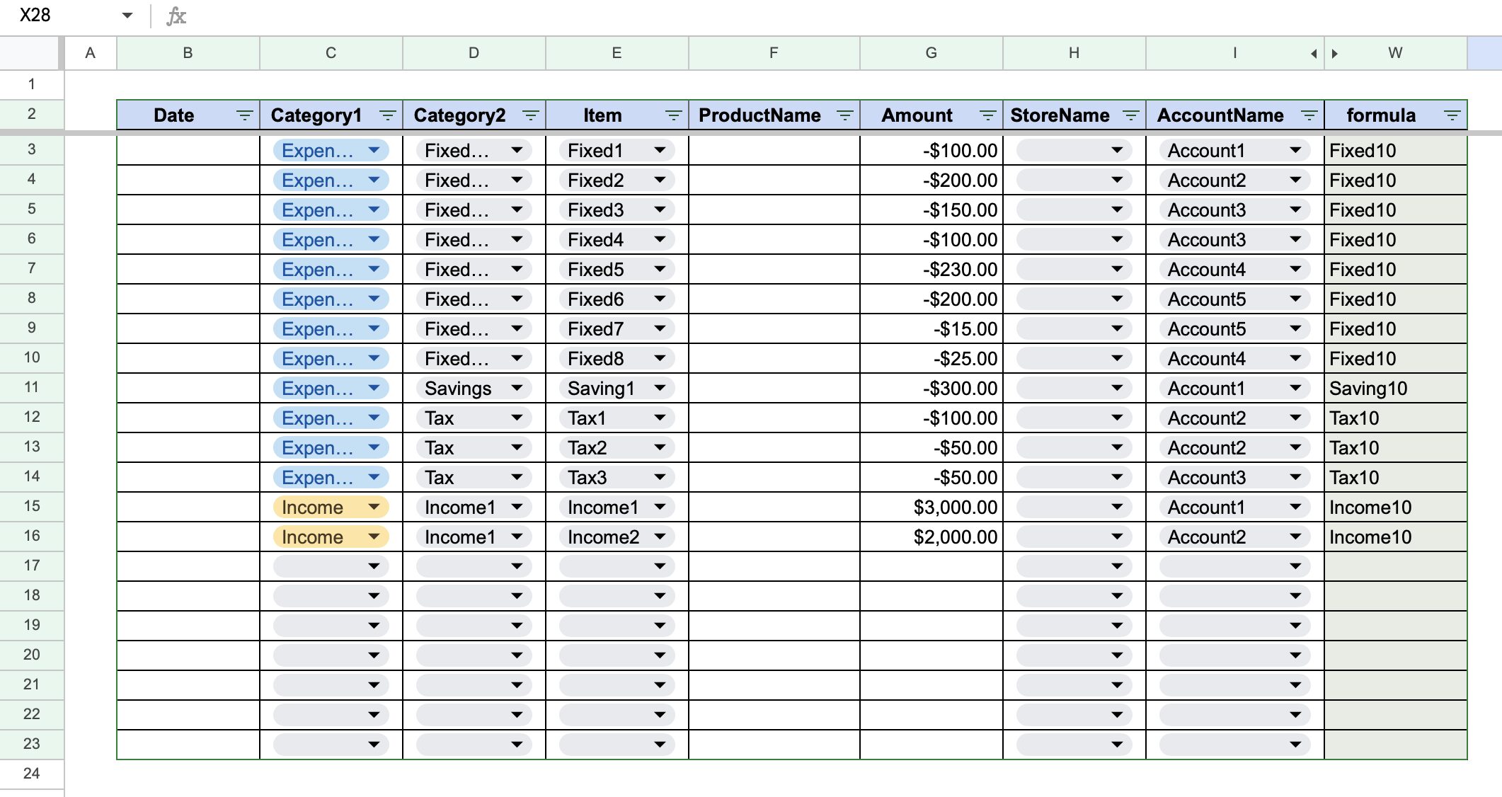
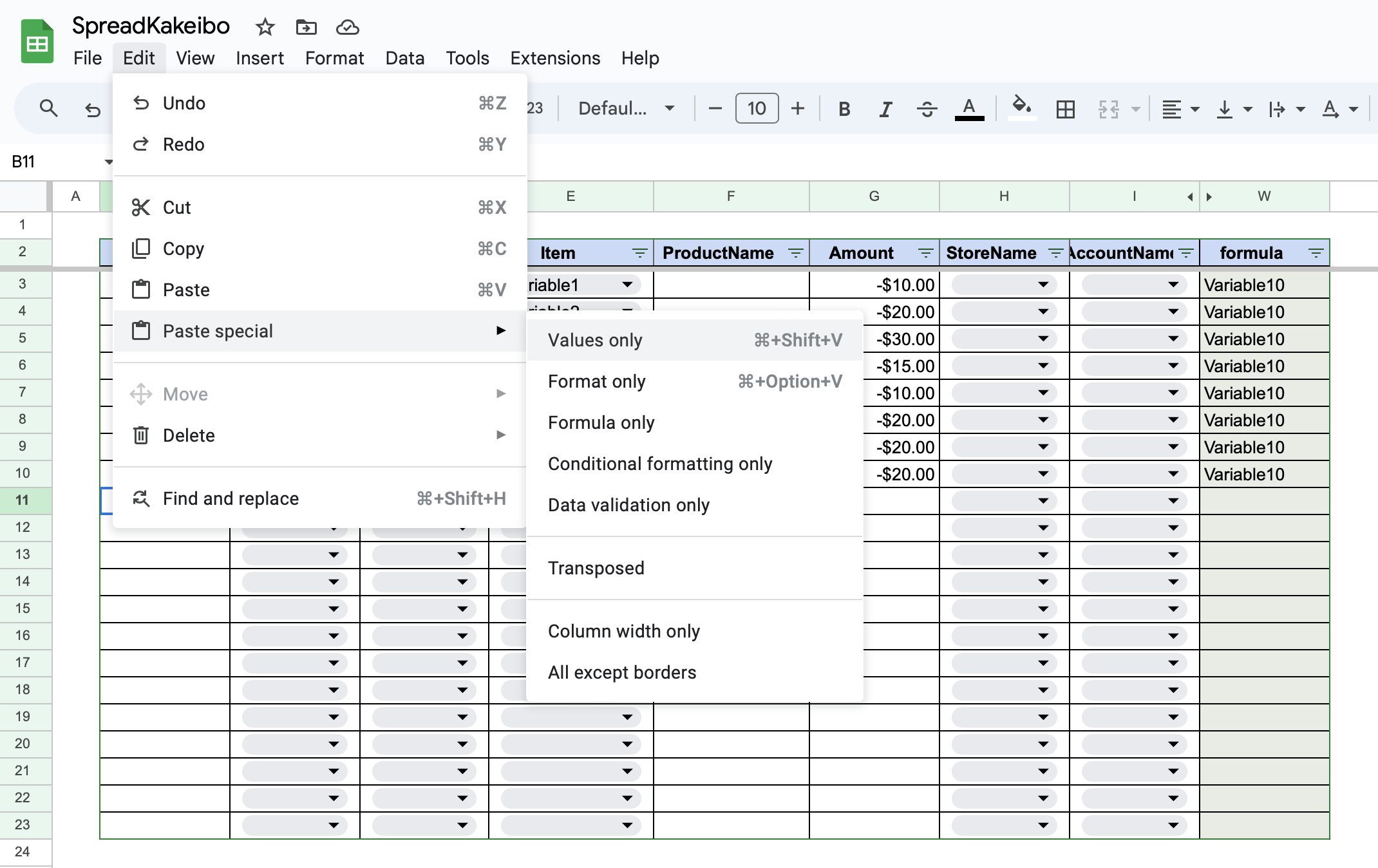
At the change of the month, paste the contents of the Fixed Expenses sheet into the Input sheet.

Select cells B3 through I16.

Do not select the heading row.

Go to the input sheet and click on the date column below the last line of input.

Click on "Edit," "Paste Special," and paste "Value Only."

If you do not select value only, an error will be displayed.

Enter the date and correct any changes to the amount or account.

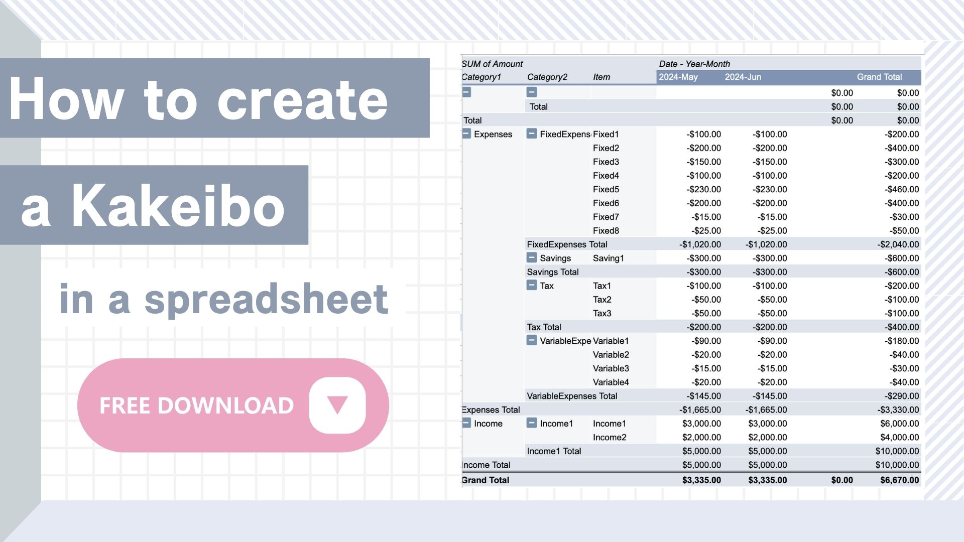
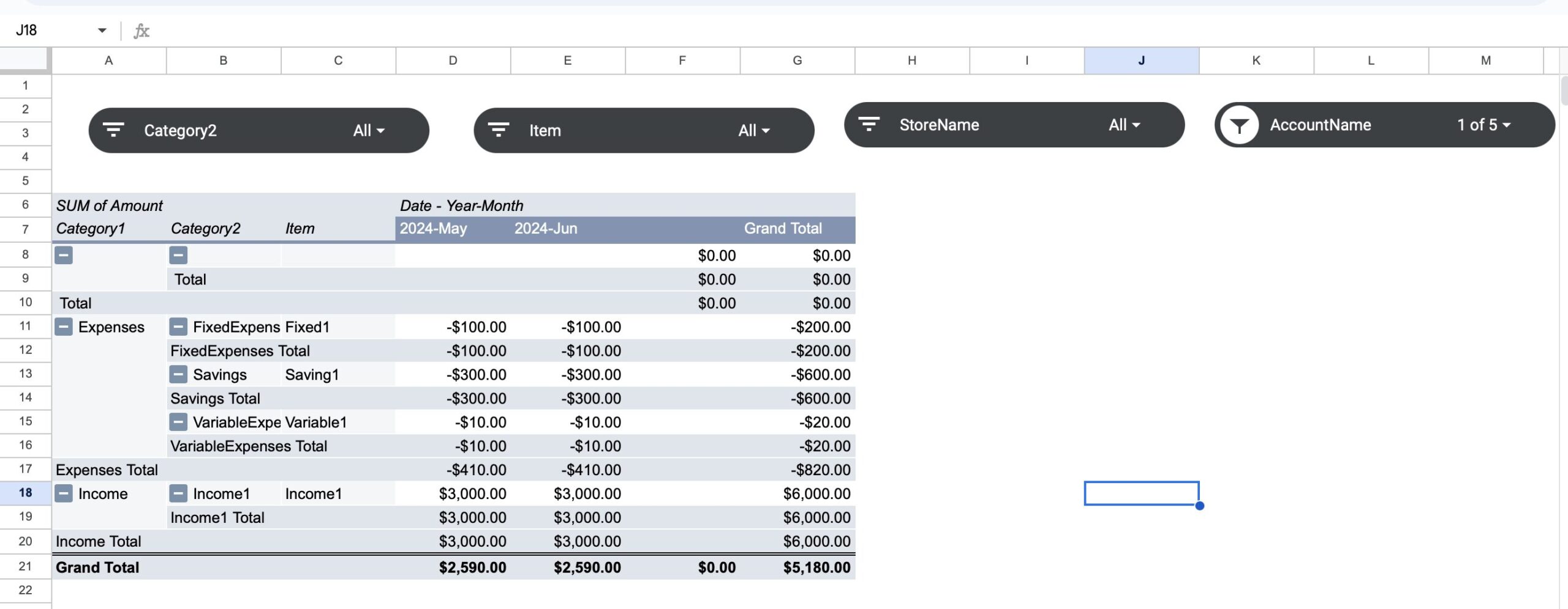
Pivot table sheet

A pivot table is created based on the data in the input sheet.

A pivot table is a table that tabulates a large amount of data by item.

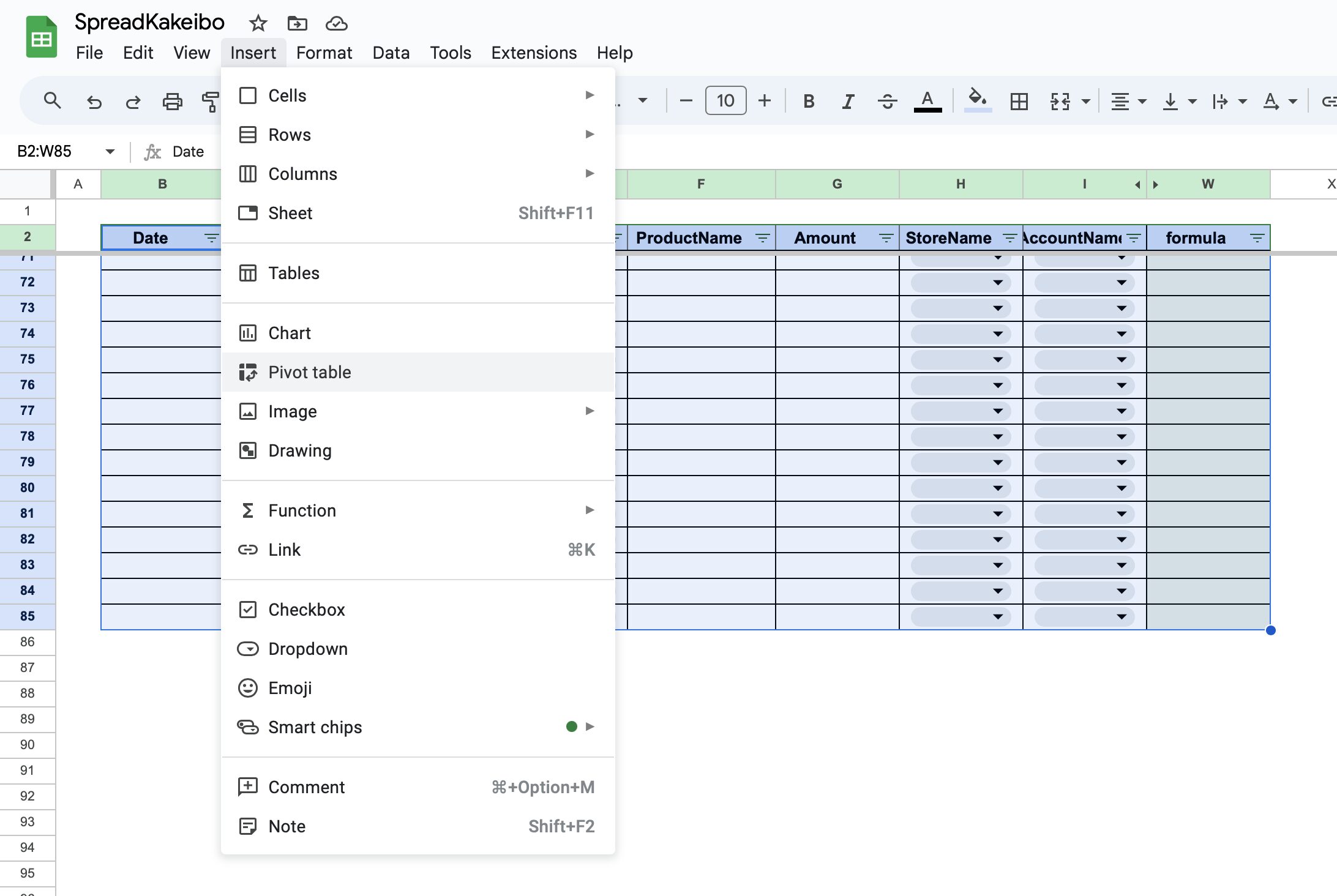
Create a Pivot Table

Select a range of input sheets.

Select a range for the table that includes heading rows and blank rows.

Click on "Insert" and "Pivot Table.

For Insert to, check "New Sheet".

For Data Range, the selected range will be displayed.

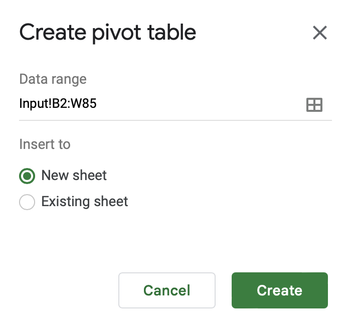
The pivot table will appear on a new sheet.

Use the Pivot Table Editor on the right to set the items.

Pivot table display items

• Rows: Category 1, Category 2, Item
• Columns: Date
• Value: Amount

Click the Add Row button and select Category 1, Category 2, and Item.

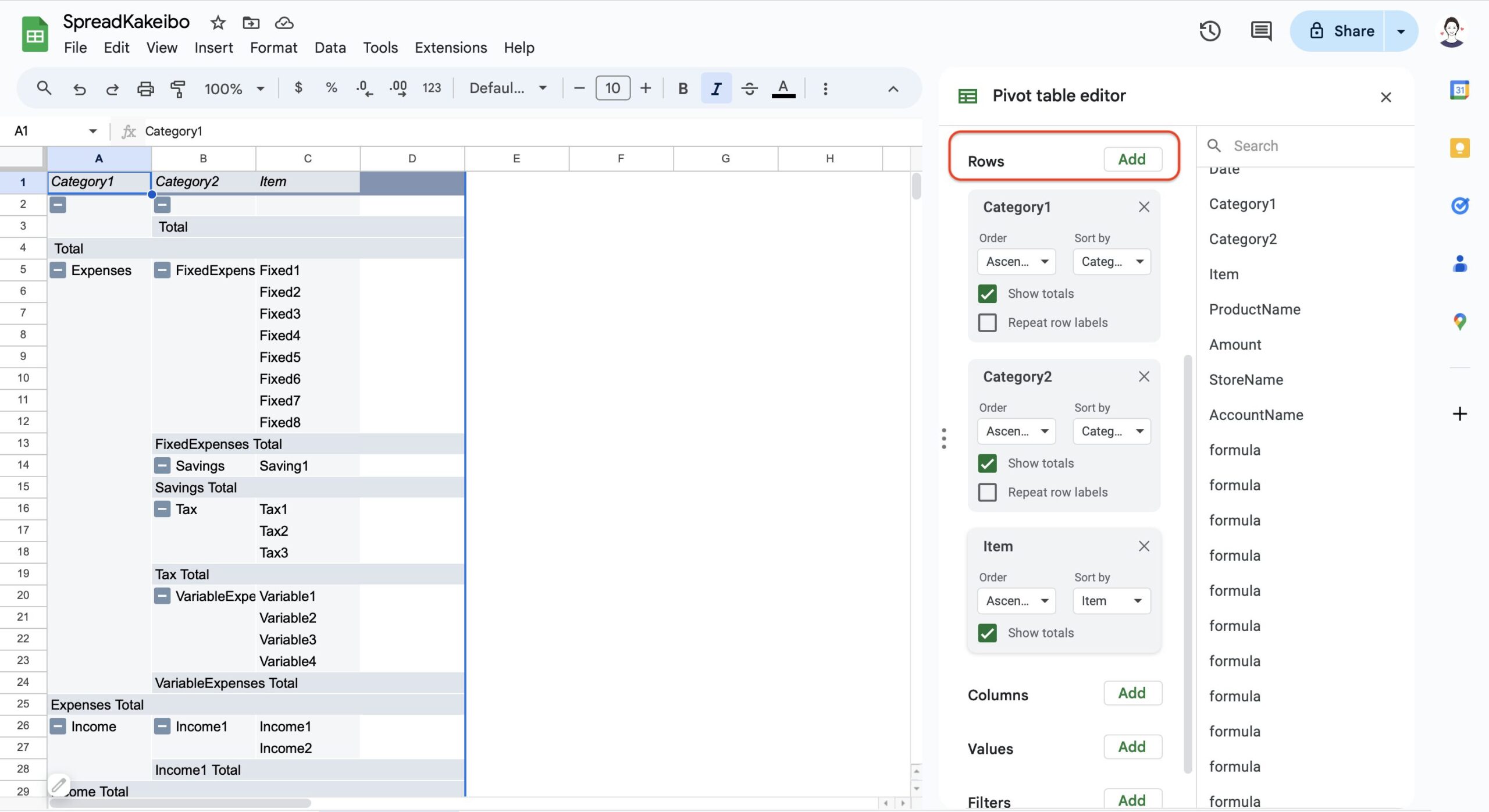
Added "Date" column and "Amount" value.

The pivot table for the display items you set will be displayed.

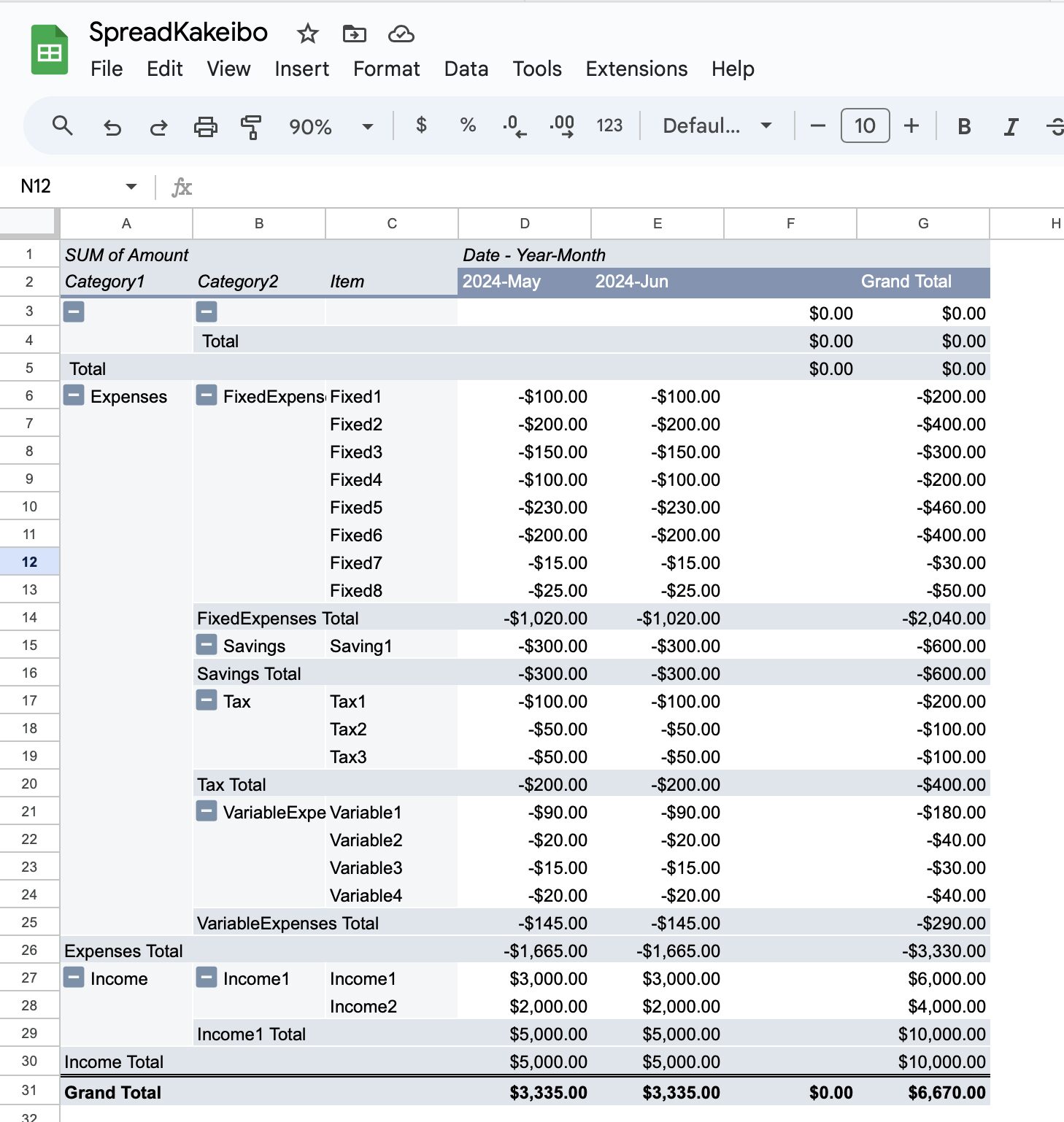
Change from view by date to view by month.

Select any date and right-click.

Select "Create Pivot Date Group" and "Year-Month.

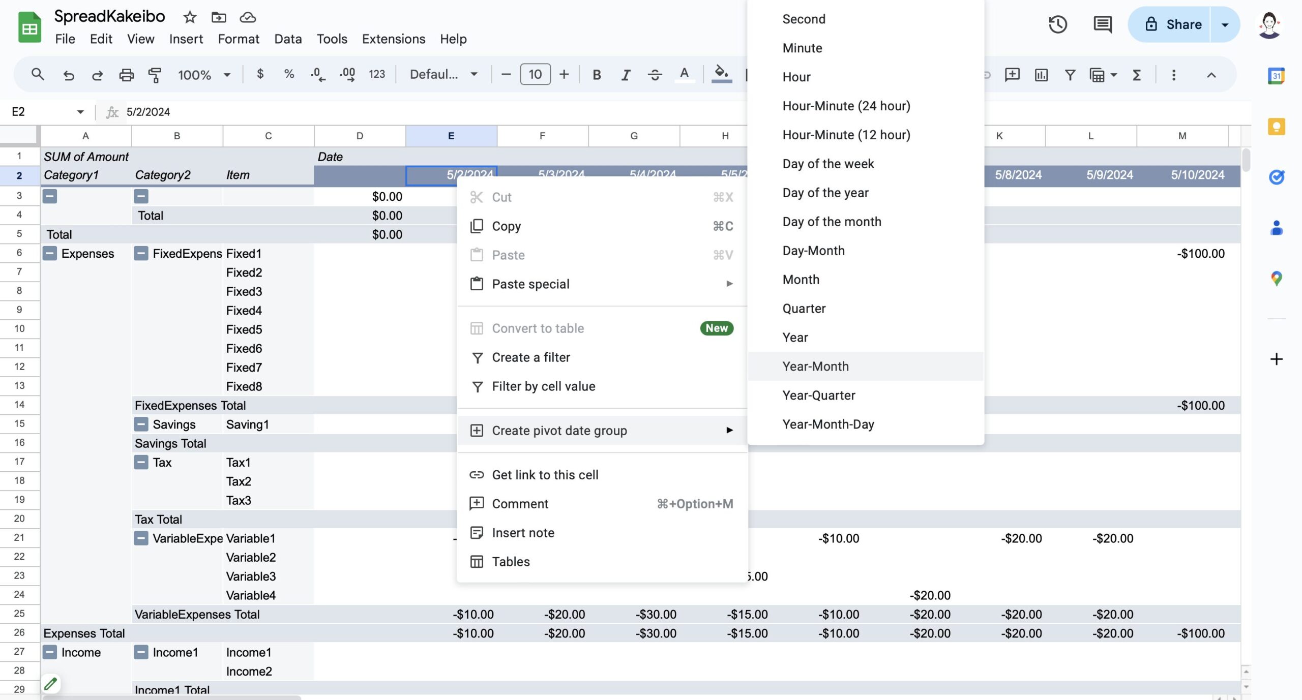
The display will be changed to a monthly display.

Creating a Slicer

You want to display the information separately by expense item, store name, account, etc.

Create a slicer for such cases.

Slicer functions

For example, you can enter a specific product name in the item name on the input sheet and display only that specific product name.

This is also useful if you want to know how much you spent on Amazon in a month or how much you spent on your credit card in a month.

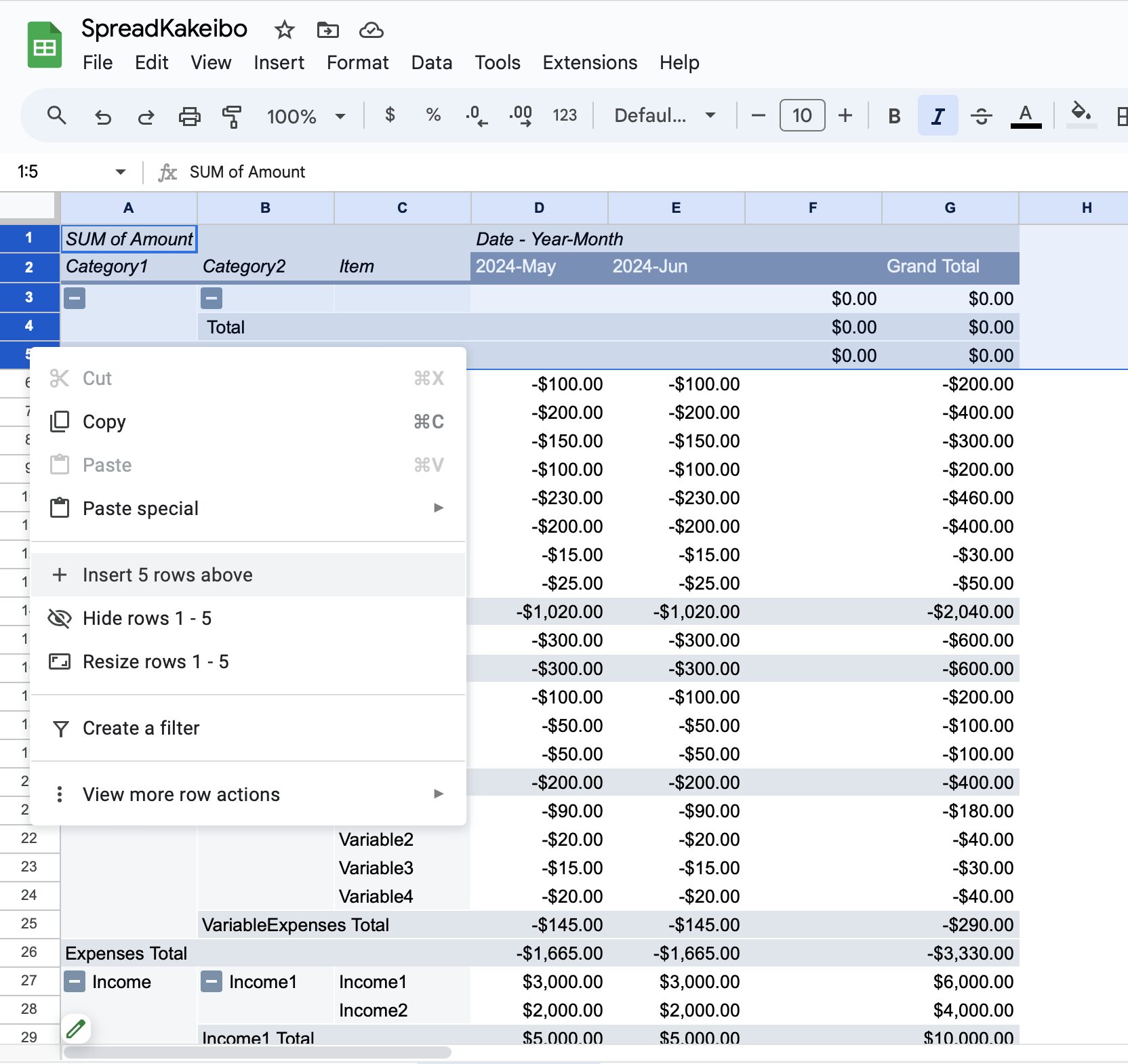
Insert Row

Add a row to make room for the slicer.

Select about the fifth row, right click, and click "Insert 5 rows above".

Select a portion of the pivot table range and right-click.

Click on "Data" and "Add a Slicer.

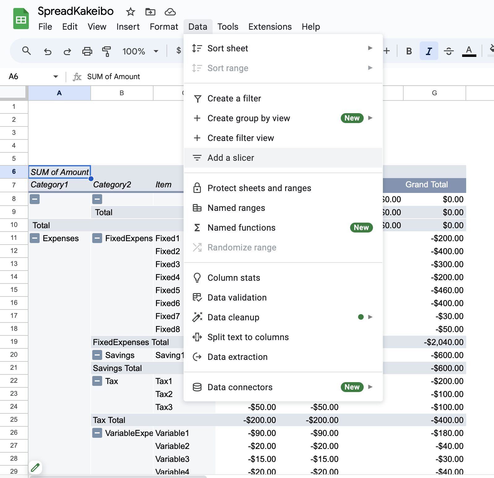
A slicer will be added and the statement "Select column first.

Select the item you wish to search.

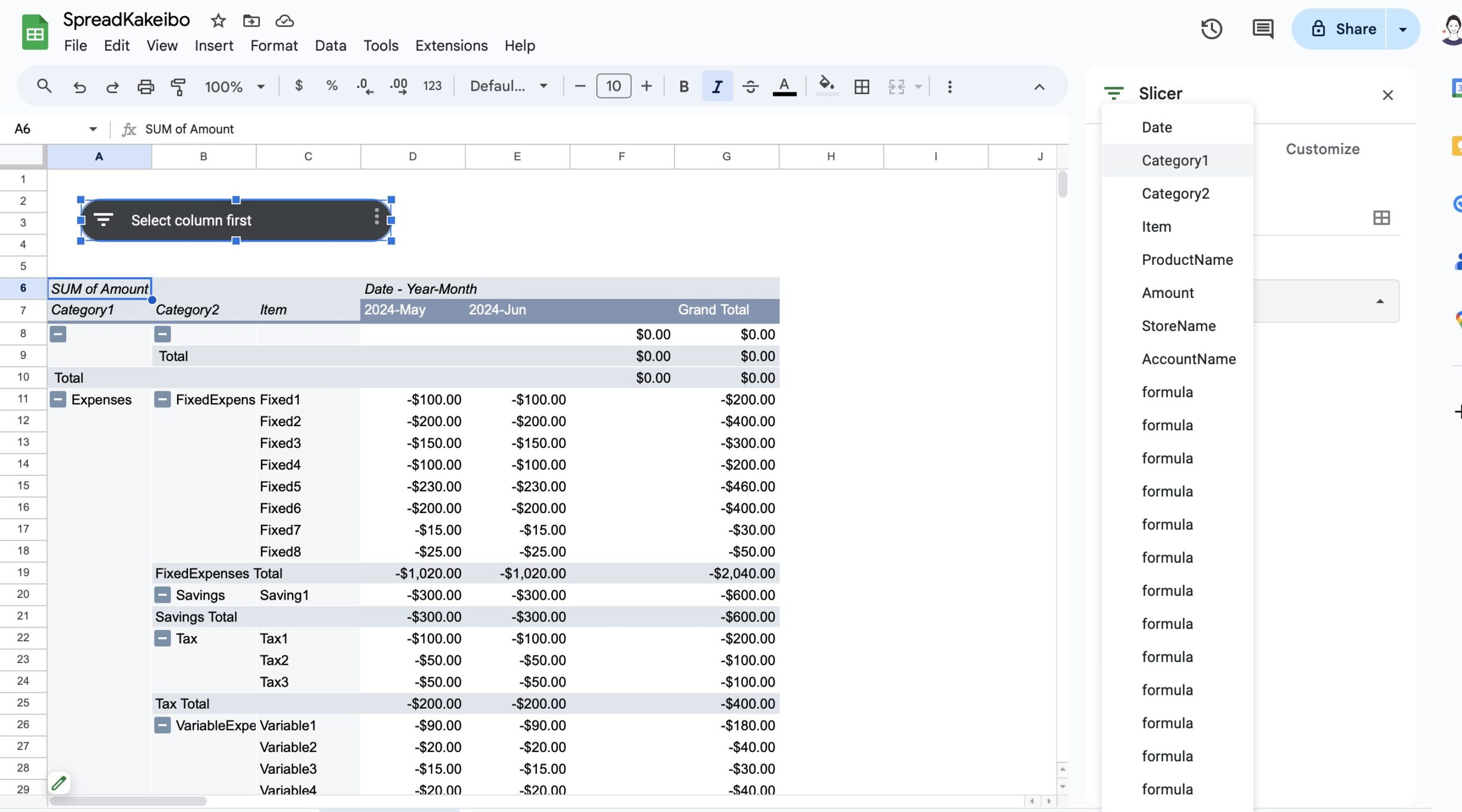
Follow the same procedure to add items you wish to search.

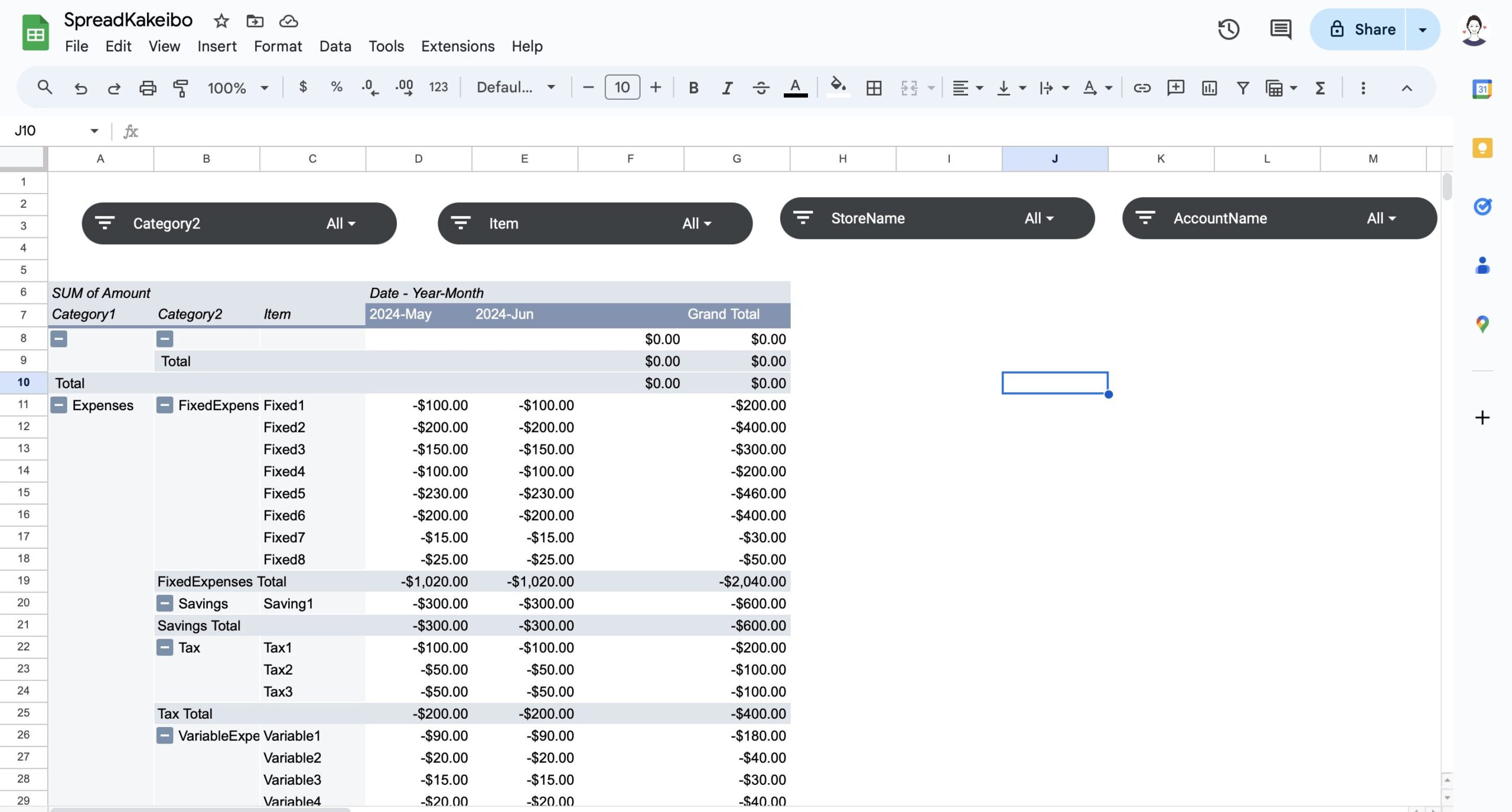
To search, click on "All" in the slicer.

After clicking "Clear," check the items you wish to search.

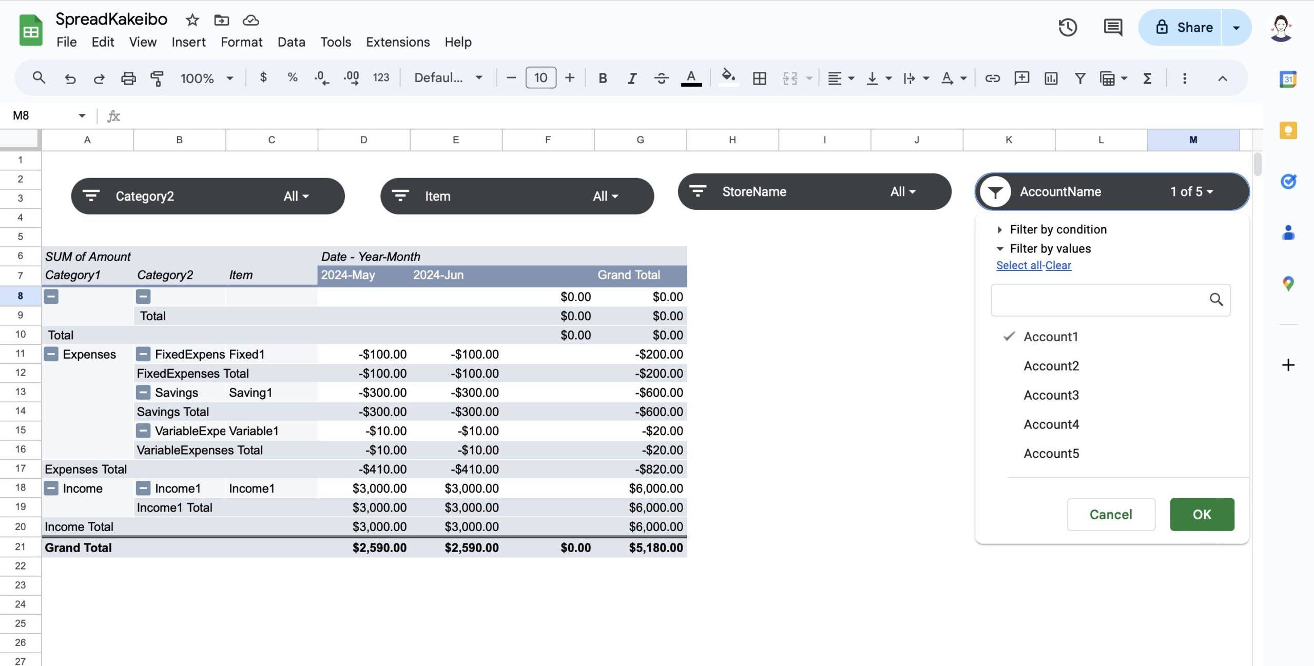
Only the specific items you searched for will be displayed.

To undo, click "Select All".

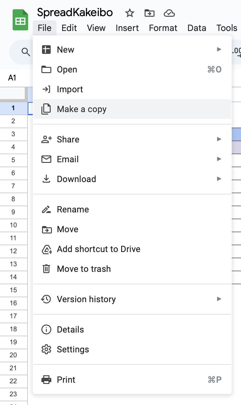
Sample Download

After downloading, please "Make a copy "of the file before use.
The downloaded file is for viewing only and cannot be edited.

The sample kakeibo may differ slightly from the template introduced here.
I appreciate your understanding.

Free download

For more information on how to use the system, click here ↓↓↓

Google Spreadsheet is also OK! Household account book with pivot table for solid analysis (free templates available)

I want to keep track of my household finances in a Google Spreadsheet.I also want to do a thorough analysis. Do you have such a ...